
The respiratory disease, COVID-19, was first reported in China’s Hubai province in 2019 and then rapidly spread across the globe. Due to its rapid spread and deadly nature, it is being characterized as one of the deadliest pandemics in history. Currently, intense interdisciplinary research into its causes, prevention, and treatments is being conducted worldwide.
Together with other scientific branches, statistics is contributing to the diagnostics, therapeutics, and public intervention in the fight against the disease.
An extremely important statistical task is to organize, summarize, and present appropriately the COVID-19 data. It must be stressed how important it is to summarize the data before the information it conveys can be properly understood. For example, daily cases and deaths are reported in the media on a daily basis, but the daily fluctuations (which can be due to many factors, such as the way the tests are collected and disseminated) do not necessarily present any new tendencies. The report of the daily cases and deaths can be misleading and a source of unnecessary worries.
In order to correct misunderstandings of this kinds, statisticians suggest using moving averages, which include 3, 5 or 7-day periods.
Suppose that we have data representing units of real estate sold during the years 1952-1982. When we have a sequence of values of a variable (units of real estate sold) taken at successive time periods, we say that we have a time series. In time series, data are given over years, months, days, and in general any unit of time.
Suppose we want to compute the five-year moving average for the data:
We take the data value for the year 1954, add to it the values for the years 1952, 1953, 1955, 1956 and divide the sum by 5. We then use the resulting average in place of the original data value for the year 1954. Similarly, we replace the original data value for the year 1955 with the average of the five data values for the years 1953, 1954, 1955, 1956, 1957. Thus, we may be able to detect the behavior of data by observing the averages of five data values at any time period instead of observing the original data values.
In a time series example, https://otexts.com/fpp2/moving-averages.html, the data represents residential electricity sales (excluding hot water) for South Australia over the years 1989 through 2008. The 5-year moving average curve (red curve) provides an estimate of the trend cycle, as it can be seen in the following graph:
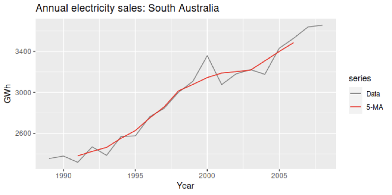
The red curve of the moving averages depicts a trend in the data in a better way than the original data.
While moving averages help in visualizing the trends in the data, they do not give information about the magnitude and variation of the trends. The statistical analysis of the trends in cases and rates of infection will help in evaluating each trend, making decisions, and reliably implementing local restrictions, particularly in case of resurgences of infection.
In 2020, D. Ison published his analysis on COVID-19 trends in data that have been collected over May 2020 through June 2020.
He obtained the data from the Center for Disease Control COVID Data Tracker website, www.cdc.gov/covid/data/tracker , and from the individual state health data repositories through the COVID Tracking Project, which receives data feeds from state health data providers several times per day www.covidtracking.com . For states that did not provide the rates of infection, these were calculated using the same data and formula used by the Center for Disease Control’s COVID Data Tracker.
The data were daily rates of cases per 100,000 individuals, collected for the U.S. and for New York, Arizona, Texas, Georgia, and Louisiana individually.
The original values were replaced with the corresponding values of moving averages.
Each of the states was selected because of a particular COVID-19 pattern in rates of cases: New York possibly passed peak infection , Arizona and Texas reported surges in cases, Georgia reported a quite stable situation, and Louisiana appeared to have an uptick in June.
The author tested statistically the about statements and concluded that some were correct, but some of them were unreliable.
The implementation, and advantages of many of the techniques used in the paper are explained below.
The Spearman Correlation coefficient and its use on COVID-19 data
The variable of interest is $rates\ of\ cases$ and varies over time. In this publication, the author considers values of the variable from April 1 through June 10, 2020, and in many instances, groups the values over the periods May 21 through June 3, 2020, June 4 through June 10, 2020, and June 6 through June 10, 2020. The statistical analysis aims at revealing a general behavior of the $rates\ of\ cases$, which can be characterized as showing a downward trend, an upward trend or neither of them.
So, the research question of the survey is to determine the trends in the data. Undoubtedly, the findings can be used in forecasting applications.
The variable of interest, $rates\ of\ cases$, is a time series since its values are taken at successive time periods.
Following a well-known technique in time series, $rates\ of\ cases$ can be considered as a dependent variable and time as an independent variable with starting date April 1.
The first step towards revealing a trend in the values of $rates\ of\ cases$ is to examine the Spearman correlation coefficient between $rates\ of\ cases$ and time. Here, the use of Spearman correlation coefficient is necessary since there isn’t any reasons to assume that the distribution of the variable $rates\ of\ cases$ is normal, in the contrary such an assumption would be wrong.
The Spearman correlation coefficient, $\ r_s$ or rho, is a non-parametric measure of the strength of an association between two variables $X$ and $Y$, i.e., it assesses how well an arbitrary monotonic function can describe a relationship between two variables. In a monotonic pattern, the variables tend to change together, i.e., the increase of the values of one variable occurs simultaneously with the increase of the values of the other variable, or with their decrease. In the former case, the Spearman correlation coefficient is positive, whereas in the later the Spearman correlation coefficient is negative. When computing the Spearman correlation coefficient, the change of the values of the variables does not occur necessarily at a constant rate.
Spearman’s rho correlation coefficient takes on values that vary between +1 (perfect positive association between the two variables) and -1 (perfect negative association).
The value of the Spearman correlation gives an insight in the strength of the association: if the correlation coefficient is close to +1 or -1 then the association is stronger.
Briefly, a significant Spearman correlation coefficient which is positive (negative) suggests an increasing (decreasing) trend. This statement can then be checked with more statistical tests.
Spearman’s correlation coefficient is similar to Pearson’s in that they both reveal monotonic trends in the data, but they have essential differences.
Particularly:
- Spearman’s correlation coefficient, as a non-parametric technique, does not make assumptions about the distributions of the variables.
- Spearman’s correlation coefficient operates on the ranks of the data.
- Spearman’s correlation coefficient describes monotonic trends of the data, and not linear trends.
Obviously, the advantages of Spearman’s correlation coefficient are that it is unaffected by the distribution of the variables, it is relatively insensitive to outlies since when dealing with ranks the magnitude of the data is not essential, and its use on ranks allows for the collection of data over irregularly spaced intervals.
One of its disadvantages is the loss of information when the data are converted to ranks.
For the calculation of the Spearman correlation coefficient ranks are assigned to the values of the variable $X$, assigning the smallest rank, i.e., 1 to the smallest in magnitude value of the variable $X$, then the rank 2 to the second smallest in magnitude value of $X$, until reaching the largest in magnitude value of $X$. The same process applies on $Y$. Then, the Spearman correlation coefficient is
$$r_s=1-\frac{6\sum d_i^2}{n^3-n}$$
where d are the differences between the paired measurements $x_i$ and $y_i$ of the two variables.
If repeated samples of size n<30 (theoretically an infinite number of samples) of the variables under examination for correlation, say $X$ and $Y$, are collected and the Spearman correlation coefficient, $r_s$, is computed for every sample, all these correlation coefficients form a distribution (this is an idea similar to the idea of the sampling distribution of the mean). The critical values of this distribution for various levels of significance are given in the so-called Spearman’s tables. The distribution of Spearman’s coefficients is used when statistical hypotheses about the monotonic associations of the variables must be checked, i.e., when the independence of variables is under question. For the correlation tests, the null and alternative hypotheses are set as:
$H_0$: There is no monotonic association between the variables.
$H_1$: There is a monotonic association between the variables.
The above pair of hypotheses specifies a two-sided test.
$H_0$: There is no monotonic association between the variables.
$H_1$: There is an increasing (or decreasing) monotonic association between the variables.
The above two pairs of hypotheses specify a one-sided tests.
The test statistic for this test is the correlation coefficient $r_s$, and the null hypothesis is rejected if the correlation $r_s$ found from the calculations based on the sample is greater than the critical value of $r_s$ for the chosen significance level. The test is performed following the strategy of any statistical test.
The above calculations are straightforward in R, where the commands used are
$cor\ (x,y,\ method=c\left(\mathrm{“spearman”}\right))$
$cor.test(x,y,\ method=c\left(\mathrm{“spearman”}\right))$
Table 2
Spearman’s correlation between the $rates\ of\ cases$ and time, for each geographical area investigated in the survey.
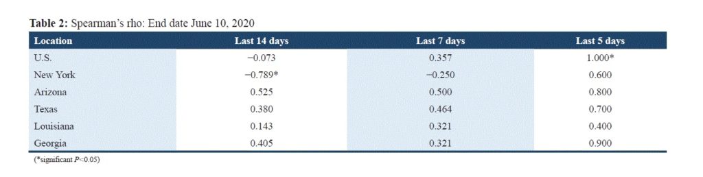
The Spearman correlation coefficient for the USA 14 days prior to June 10th (from May 27 through June 10) shows negative association between $rates\ of\ cases$ and $time$, but it is so weak that it is not possible to state if there is a decrease in the rates of cases over time. Toward recent data the association becomes positive and stronger. Specifically, the last 7-day period rho is equal to +0.357, suggesting an increase in cases over time, and the last 5-day period is equal to 1 and statistically significant, indicating a perfect positive association between the cases and time.
In New York, the situation raised some concerns since a strong negative association becomes moderately positive when moving toward latest data. Specifically, the last 14-day period the Spearman coefficient is negative and statistically significant, suggesting a strong decrease of cases over time, but it increases toward recent data, and the last 5-day period it exhibits a strong value although not statistically significant. These findings lead to the assumption of an increase of cases.
In Louisiana, the ranking is not directly correlated with time, and the associations appear to change from slightly positive to moderately positive but with no statistical significance, although Louisiana was reported to have a definite uptick in June.
In Texas and Arizona, the correlation coefficients are positive and moderately strong. The last 5-day period rho exhibits an increase, suggesting a positive trend in the data.
Table 3
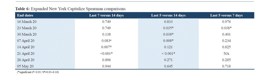
Expanded New York Spearman’s correlation coefficients
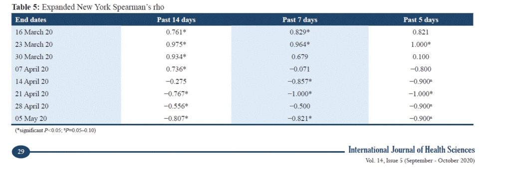
The expanded correlation coefficients describe a concrete trend in the COVID-19 data for New York. In the beginning, using as the end date the 16th of March and moving backward 2-week , 1-week and 5-day periods, strong statistically significant positive associations occur. The same pattern, but with stronger statistically significant correlations, appears when 23rd of March is considered as the end date. Then the correlations start to weaken, and toward recent days strong negative correlations appear, often statistically significant. These findings lead to the assumption that New York experienced the transition from strong increases in $rates\ of\ cases$ to peak values and to decreases.
This statement must be examined by using other statistical tests.
Comparisons of nonparametric correlations
It is useful to compare the Spearman correlations in order to understand better the strength of the relationship between the variables.
However, the distribution of r over all possible samples of the two variables, i.e., the sampling distribution of r, is symmetric under the condition the population correlation, $\varrho$, is equal to zero.
If the Spearman population correlation, $\varrho\ $, is equal to zero and the two variables have a bivariate normal distribution or if the sample size n is sufficiently large, then r has a normal distribution with mean equal to zero, and $t=\frac{r}{s_r}$ where $s_r=\sqrt{\frac{1-r^2}{n-2}}$ follows a t-distribution with n-2 degrees of freedom.
If we cannot make assumptions about the distribution of the variables, we compute the Fisher transformation of the Spearman’s correlation $ r_s\ $ as follows:
$r_s^\prime=0.5\ast ln\frac{1+r_s}{1-r_s}$
Suppose $\varrho_X=\varrho_Y$, $X$ and $Y$ have joint bivariate normal distribution, or the size of the samples is sufficiently large. If $r_{s1}$ and $r_{s2}$ are the Spearman correlation coefficients of two independent samples and $r_{s1}^\prime$ and $r_{s2}^\prime$ are the corresponding Fisher transformations, then the statistic $z=\frac{r_{s1}^\prime-r_{s2}^\prime}{s}$ where $s=\sqrt{\frac{1}{n_1-3}+\frac{1}{n_2-3}}$ follows a standard normal distribution.
Table 4
Comparison of Spearman’s correlation coefficients based on samples chosen over various time periods.
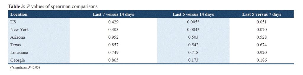
There are only two significant results: The first one is related to the whole US and refers to the difference of correlations 14 days prior to the end date and 5 days prior to the end day. The comparison between the Spearman coefficients points to an increase in $rates\ of\ cases$ over the last 5-day period and aligns with the results related to the correlation coefficients described in Table 2. The second result is related to the New York cases over the same periods. The statistically significant differences between the Spearman correlation coefficients for the cases over the last 5 versus last 14 days reinforces the conjecture about the increase in cases for New York and the USA. On the other hand, the comparisons of the correlation coefficients related to the other states do not exhibit any statistically significant difference between them, although it was reported that in Louisiana there was a considerable increase in $rates\ of\ cases$.
Table 5
Comparison of Spearman’s correlation coefficients based on New York samples chosen over various time periods
For the expanded rates of cases in New York the author chose a longer period from March 3 through May 5. He divided the time into 14-day, 7-day and 5-day periods. In many cases a statistically significant difference of Spearman coefficients is presented for $rates\ of\ cases$ over the 14-day period and the 5-day period before the end day. The statistically significant differences between the Spearman correlations together with the opposite signs of Spearman correlations for data over time periods given in Tables 2 and 3 indicated that possibly there are some trends in the data. More statistical tests are necessary to reveal the existence of trends since the correlation coefficients shown the abovementioned strong associations.
Mann-Whitney U test
Subsequently, the author wanted to examine if the rates of cases over the 14-day period of May 21 through June 3, 2020, are similar to the rates of cases over the 7-day period of June 4 to June 10, 2020. Statistically speaking, he wanted to examine if the mean of the rates of cases over the first period is equal to the mean of the rates of cases over the second period. This is a typical case of a t-test , but its assumptions are not met: the variables under examination are not normally distributed which could justify the use of a z or t-distribution based on the central limit theorem. The equivalent of t-test when its assumptions are not met is the Mann-Whitney U test, often named as Wilcoxon rank sum test. This is a non-parametric test that examines the equality of two populations in terms of a number of central tendency (mean or median). The test can be implemented even for small samples, under the following conditions:
- The observations can be divided into two groups/categories in a clear and well-defined way. In our statistical study, all the observations belong to two different groups namely, the ones that were recorded over the time interval of May 21 through June 3 and the ones that were recorded over June 4 through June 10.
- The observations must be independent. In our statistical study, there is no relationship between the data collected over the period of May 21 through June 3 and the data collected over the period of June 4 through June 10 since there are different participants in each group with no participants belonging to both groups.
- The observations must be measured at ordinal, interval, or ratio level. In our statistical study, $rate\ of\ cases$ is a continuous variable.
Usually, a Mann-Whitney test is two sided , and the null hypothesis asserts that the two population (from where the two samples of observations are drawn) are equal. In our statistical study, the author was interested in detecting a positive or negative shift in one population as compared to the other, so he specified directionality in the alternative hypothesis and worked with one-sided tests.
For the running of the test, the observations are all grouped together and are ranked, beginning with the rank 1 for the smallest observation in magnitude. Then a test statistic U is computed based on the ranks and U follows the U-distribution when the samples sizes are small.
For larger samples (greater than 20) the test statistic U follows a normal distribution with mean $\frac{n_1\ast n_2}{2}$ and standard deviation $\sqrt{\frac{n_1\ast n_2\ast(n_1+n_2+1)}{12}}$, where $n_1$ is the size of the first sample and $n_2$ is the size of the second sample.
The standard deviation changes if there are ties and becomes:
$$ \sqrt{\frac{n_1\ast n_2}{12}\ast(\left(n+1\right)-\sum_{1}^{k}{\frac{t_g^3-t_g}{n(n-1)})}}, $$
where $n=n_1+n_2$, k is the number of tied groups,
and $t_g$ the number of values in each tied group.
To run the test in R, use the command $wilcox.test(x,y)$
Suppose we want to compare the following two samples for which there are no assumptions about the distribution of their populations.
First sample:
8, 2, 6, 10, 9, 2, 8, 10, 1, 6
Second sample
6, 3, 7, 7, 6, 1, 6, 8, 2, 4
Necessarily the Mann-Whitney test must be implemented to compare numbers of central tendency with the following test hypotheses:
$H_0$: The two populations are equal.
$H_1$: The two populations are not equal.
If the null hypothesis is true, then the samples are drawn from similar populations, i.e., populations with similar means and shapes.
The first calculation for this test is to assign ranks to the data: the data of both samples are combined together and arranged in increasing order. Thereafter ranks must be assigned to each data value beginning with the smallest in magnitude which will be ranked as 1, the second smallest will be ranked as 2 until reaching the greatest value in magnitude. If there are some data values that are equal, they are tied, the midpoint of their rankings must be re-assigned to every one of these values. In our example, the data value 1 is found in the first and the second sample. Since the value 1 is the smallest in magnitude and appears twice, the ranks 1 and 2 are assigned to each of the values. The average of the assigned ranks is $(1+2)/2=1.5$. So, the rank 1.5 is re-assigned to each one of the data values in both sample. If a data value is found in the samples more than two times, then firstly successive numeric ranks must be assigned to all the (equal) values and subsequently the midpoint of the ranking must be re-assigned to each one of them.
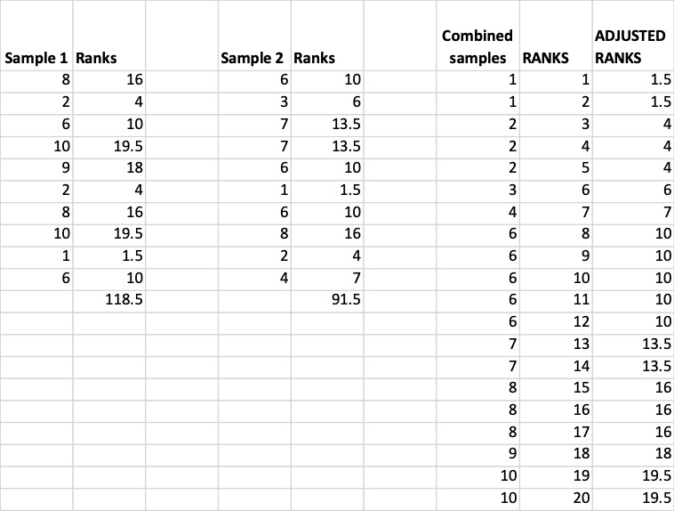
The sum of the ranks $R_1$ for the first sample, and $R_2$ for the second sample, are computed:
$R_1=118.5$ and $R_2=91.5$
Subsequently, the numbers
$U_1=n_1\ast n_2+\frac{n_1\left(n_1+1\right)}{2}-R_1$ and $U_2=n_1\ast n_2+\frac{n_2\left(n_2+1\right)}{2}-R_{12}$ must be computed,
where $n_1$ and $n_2$ are the sizes of the first and second sample respectively:
$U_1=n_1\ast n_2+\frac{n_1\left(n_1+1\right)}{2}-R_1=10\ast10+\frac{10\ast11}{2}-118.5=36.5$
$U_2=n_1\ast n_2+\frac{n_2\left(n_2+1\right)}{2}-R_{12}=10\ast10+\frac{10\ast11}{2}-91.5=63.5$
The test statistic for the Mann-Whitney test is the smallest between the Us, so 36.5. It has to be compared against the critical value in the U distribution: since the sample sizes of each sample is 10, at a 95% level of confidence $U_{critical}\left(10,10\right)=23$ (the critical value can be found by the tables of U distribution).
For any Mann-Whitney U test the theoretical range of U is from 0 to the number $n_1\ast n_2$. For the U-distribution and the Mann-Whitney U test there is a $pronounced\ differentiation$ related to the other statistical tests:
if the observed value of U is less than or equal to the critical value, we reject the null hypothesis and if the observed value is greater than the critical value, we do not have reasons to reject the null hypothesis.
In this example since $36.5>23$, then based on the above sample there is no reason to reject the null hypothesis.
If we run the test in R, the results are exactly the same. The test statistic W is equal to the number $U_2$ found above calculated by hand. R chooses as test statistic the greatest among the $U_is$ because the reverse decision rule is followed:
Figure 2
R-output for Mann-Whitney test
> x
[1]  8  2  6 10  9  2  8 10  1  6
> y
[1] 6 3 7 7 6 1 6 8 2 4
> wilcox.test(x,y)
Wilcoxon rank sum test with continuity correction
data:  x and y
W = 63.5, p-value = 0.32
alternative hypothesis: true location shift is not equal to 0
Warning message:
In wilcox.test.default(x, y) : cannot compute exact p-value with ties
Table 6
Mann-Whitney test for equality of the rates of cases over two different time periods
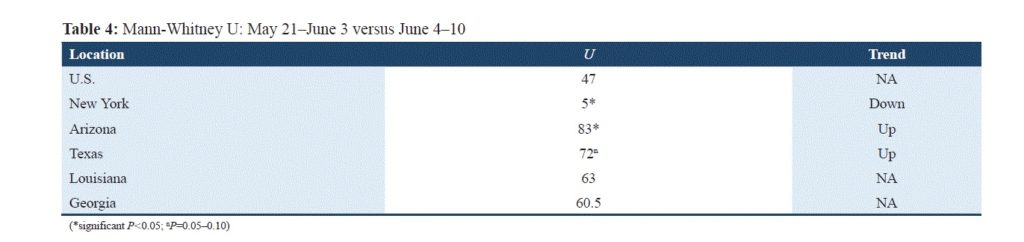
The author conducted a one-sided Mann Whitney U test for each state and for the whole country separately. For each of the tests, the hypotheses are set as:
$H_0$: The two populations during the periods May 21-June3 and June3-June 10 are equal.
$H_1$: The two populations during the periods May 21-June3 and June3-June 10 are not equal.
For each of these tests, if the null hypothesis is true then we would expect to see similar rates of cases over the first time period of May 21 through June 3, and over the second of June 4 to June 10, and also expect larger and smaller rates of cases in both samples. If the null hypothesis is rejected, an increasing or decreasing trend would appear in the second period.
For Arizona, Texas, and New York the observed rates of cases consist evidence of statistically significant differences in both population (over the first and the second time period).
More specifically, in Arizona there is an increase in the rates of cases over the 7-day period of June 4 through June 10, related to the rates of cases over the 14-day period of May 21 through June 3, and this result is statistically significant at a 5% level of significance.
The author found a similar statistically significant result for Texas, but for a lower level of significance and equal to 10%.
In contrast, the rates of cases over June 4 through June 10 are significantly decreasing related to the rates of cases over the period of May 21 through June 3 at 5% level of significance, in New York.
So, these findings reinforce the conjectures we made when working on Spearman’s correlation for the same data: examining Spearman’s correlations, a lurking uprising trend was hypothesized for New York, although for Texas and Arizona the positive and incrementally increasing Spearman’s coefficients gave us the impression of an increase in the cases. The Mann-Whitney U test reveals statistically significant differences among the rates of cases over May 21 through June 3 and June 4 through June 10, for the three states.
Mann-Kendal test and Sen’s slopes
Another test that is recognized as being appropriate to detect the increasing or decreasing trend in data collected over time is the Man-Kendall test. After running this test, particularly if its null hypothesis is rejected, the computation of Sen’s slope will shed light on data’s behavior.
Man-Kendall test is a non-parametric technique, i.e., distribution free technique, which requires that the data be neither autocorrelated nor collected seasonally.
The null hypothesis, $H_0$, for this test assumes that there is no monotonic trend in the data, and it is tested against the alternative hypothesis, $H_1$, that assumes that there is a monotonic trend (i.e., the data are not randomly ordered over time).
Apart from the fact that the Mann-Kendall test confirms the dependence of the data when the null hypothesis is rejected, additionally it reveals the monotonic nature of the trend: the sign of the test statistic asserts whether the trend is increasing (the Mann-Kendall test statistic is a positive number) or decreasing (the Mann-Kendall test statistic is a negative number).
To calculate the Mann-Kendall test statistic, S, the differences of every data value minus all former data values must be computed, i.e., the differences between later and earlier data. Every one of these differences will be represented by -1, if the difference is smaller than zero, +1, if the difference is greater than zero, and 0, if the two data values are equal, i.e., they are tied. Then the sum, S, of all negative and positive units must be computed:
$S=\sum_{i=1}^{n-1}\sum_{j=2}^{n}{sign(x_i-x_j})$,
where $sign\left(x\right)=\left[\begin{matrix}+1, & if & x>0\\ 0, & if & x=0\\ -1, & if & x<0\ \end{matrix}\right]$
With inspection it becomes clear that, if the number S is positive then the observations that appeared later in the time series are larger than those that appeared earlier. Mathematically speaking, the magnitude of the data that appeared later are relatively larger and they are plotted higher in the y-axis, so the trend is increasing, while the reverse is true when S is a negative number. For ties such conclusions cannot be made.
Suppose the number of data is greater than 10, and we collect all possible samples of data over the same time interval. For every one of these samples, we compute the corresponding test statistic S. Then all those numbers S are normally distributed with mean equal to zero and variance equal to:
$\sigma^2=\frac{1}{18}\ \left[n\left(n-1\right)\left(2n+5\right)-\sum_{1}^{g}t_p\left(t_p-1\right)\left(2t_p+5\right)\right],$
where g is the number of tied groups, and
$t_p$ the number of (equal) values in the pth tied group.
Then the standard test statistic z:
$z=\left[\begin{matrix}\frac{S-1}{\sqrt{\sigma^2}}, & if & S >0\\ 0, & if & S=0\\ \frac{S+1}{\sqrt{\sigma^2}}, & if & S<0\ \end{matrix}\right]$
follows a standard normal distribution.
After the sampling distribution of S has been established, the Man-Kendall test can be run (by hand) following the implementation of any statistical test: if the test is two sided, so the alternative hypothesis asserts that there is a monotonic trend generally, the absolute value of the test statistic z computed based on the given time series will be compared to the critical value $z_{\alpha/2}$, where $\alpha$ is the chosen level of significance (or equivalently the probability $P(\left|z\right|>z_{\alpha/2})$ must be compared to the half of the level of significance). If $\left|z\right|>z_{\alpha/2}$ (or equivalently $P\left(\left|z\right|>z_\frac{\alpha}{2}\right)<\alpha/2)$, then the null hypothesis is invalid implying that the trend is significant, i.e., there is a trend in the data. If the test is one sided, so the alternative hypothesis asserts that there is an increasing (or decreasing) trend, then z has to be compared with $z_\alpha\ $ (or equivalently the probability $P\left(z>z_\alpha\right)$ with a).
To run the test in R, firstly install the trend package developed by Thorsten Pohlert with the command $install.trend$ and then use the command:
$mk.test(x,\ alternative=c(“greater”,“smaller”,“two.sided”)$ that will give the results of a one-sided or two-sided test, depending on the choice.
When R runs the Mann-Kendall test another statistic can be obtained which is Kendall’s tau.
Kendall’s tau is a non-parametric measure of correlation between two variables, $X$ and $Y$, similar to Spearman’s rho correlation since both assess statistical association based on the ranks of the data and take on values between -1 and 1. If Kendall’s tau is a positive number close to +1 this is an indication of a strong association of high values of $X$ with high values of $Y$; although if it is a negative number close to -1 this is an indication of a strong association of high values of $X$ with low values of $Y$. Additionally, Kendall’s tau reflects the strength of the relationship between the two variables.
Its sign, which is the same as the sign of S for Mann-Kendall test, shows the nature of the trend (i.e., increasing or decreasing). To compute Kendall’s tau coefficient we proceed as follows: for every pair of observation ${(x}_i,y_i)$ all (timely) subsequent observations of this pair are considered, and the number of concordant and discordant observations is recorder; an observation ${(x}_j,y_j)$ is concordant with ${(x}_i,y_i)$ if the order between $x_i$ and $y_i$ is same as the order between $x_j$ and $y_j$; otherwise, if the order is different the couples are called discordant. For example, the couple (3 ,4) is concordant with (10, 12) since the order between the couples of the first couple, 3<4, is the same to the order between the elements of the second couple 10<12. Also, (3,4) is discordant with (2,1), because 3<4 but 2 is not smaller than 1.
Kendall’s tau is then given by:
$$\tau=\frac{n_c-n_d}{n(n-1)/2},$$
where n is the total number of (paired) observation,
$n_c$ is the total number of concordant observations,
$n_d$ is the total number of discordant observations.
There are some versions of Kendall’s tau, some of them correct for ties in the data and some others require that the data be free of ties. One variant of tau adjusted for ties, used by almost all software is Kendall’s tau $\beta$:
$$\tau_\beta=\ \frac{n_c-n_d}{\sqrt{(n_0-n_1)(n_0-n_2)}},$$
where $n_0=n(n-1)/2$,
$n_1=\sum_{i} t_i(t_i-1)/2$ = number of tied values in each $t_i$ group for the first quantity,
$n_2=\sum_{j} t_j(t_j-1)/2$ = number of tied values in each $t_j$ group for the second quantity.
Suppose the number of data is greater than 10, and we collect all possible samples of data over the same time interval. For each of these samples we compute the corresponding coefficient $\tau_\beta$. Then all those numbers $\tau_\beta$ are normally distributed with mean equal to zero and variance equal to:
$\sigma^2=\frac{2(2n+5)}{9n(n-1)}$
The normalized test statistic:
$z=\frac{3\ast\tau\ast\sqrt{n(n-1)}}{\sqrt{2\ast(2\ast n+5)}}$
roughly follows a standard normal distribution.
After the sampling distribution of $\tau$ have been established, the Man-Kendall test can be run (by hand) following the standard strategy of implementation of any statistical test: the null hypothesis of the test assumes that there is no association between the variables, i.e., $\tau=0$, and the absolute value of the test statistic z computed based on the given time series will be compared to the critical value $z_{\alpha/2}$, where $\alpha$ is the chosen level of significance (or equivalently the probability $P(\left|z\right|>z_{\alpha/2})$ must be compared to half of the level of significance). If $\left|z\right|>z_{\alpha/2}$ (or equivalently $P\left(\left|z\right|>z_\frac{\alpha}{2}\right)<\alpha/2)$, then the null hypothesis is invalid implying that there is an association between the two variables.
For Kendall’s correlation coefficients as rule of thumb we accept that if $ \left|\tau_\beta\right|>0.35\ $ there is a quite strong association between the variables.
Differences between Kendall’s and Spearman’s correlations:
- The distribution of the correlation coefficients $\tau_\beta$ converges to normal distribution faster (so for smaller sample sizes) than the distribution of $r_s$.
- Kendall’s Tau distribution exhibits smaller standard errors than Spearman’s rho distribution.
- The confidence intervals and consequently the p-values for \tau_\beta tend to be more reliable than for $r_s$
Absolute values for Kendall’s tau coefficients tend to be smaller than for Spearman’s when both have been calculated for the same data: $ \left|\tau_\beta\right|\le 0.7\ \left|r_s\right|$
When a trend is detected in the data, i.e., the null hypothesis of Mann-Kendell’s test is rejected, the nature of the trend which is given by the sign of the Mann-Kendall test statistic helps get an idea about the shape of the time series, but it is not enough. The magnitude of the trend is needed to understand the “steepness” of the time series.
If there is a linear relationship in the data, so a straight line is passing close enough by the vast majority of data, then the magnitude of the trend is estimated by the slope of the line which is the coefficient of the independent variable in the equation of the line and is calculated by the method of least squares.
When the trend in the data is not linear, like in our example, obviously we cannot calculate the slope of a line. Sen suggested to calculate a kind of slope of the trends that are presented in the data over a time interval and then to find their median. The median can be used as an estimator of the slope of the trend over the given time interval, and gives the magnitude of the trend, i.e., how much the trend is increasing or decreasing per unit time:
$ \beta=median\left(\frac{x_j-x_i}{j-i}\right),\ for\ all\ j>i $
So, if b is positive (negative), the trend is increasing (decreasing), and the value of the median gives the increase (decrease) per unit time.
The R command $sens.slope(x,\ conf.level=)$ computes the slop of Sen at the desired confidence level.
Table 8
Mann-Kendall tests and Kendall’s correlations for the New York data over various time periods
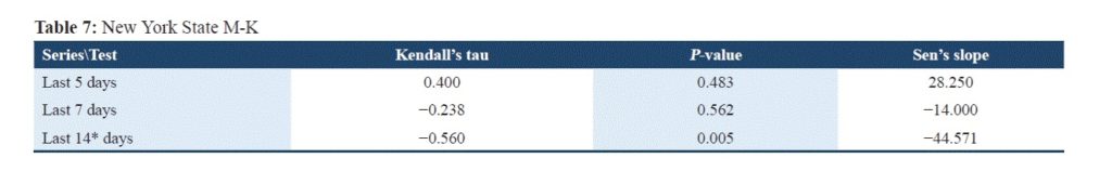
After running the Mann-Kendall tests and computing the Kendall correlation coefficients for the New York data exclusively, the author depicted his results in the above table.
The author ran 3 Mann-Kendall tests separately:
- $H_0$: There is no monotonic trend in the data over the last 14-day period.
$H_1$: There is a monotonic trend in the data over the last 14-day period. - $H_0$: There is no monotonic trend in the data over the last 7-day period.
$H_1$: There is a monotonic trend in the data over the last 7-day period. - $H_0$: There is no monotonic trend in the data over the last 5-day period.
$H_1$: There is a monotonic trend in the data over the last 5-day period.
The p-value of each of these test is the probability of finding a Mann-Kendall test statistic greater than or equal the statistic the author computed based on the New York data, under the condition the null hypothesis is true.
The p-value of each of the three tests is depicted in the third column of the above table.
The p-value of the first test is equal to 0.005, smaller than the threshold 0.05, and it means that there is an extremely small probability of getting a Mann-Kendall test statistic equal to the test statistic computed on the New York sample under the condition of the independence of data. Consequently, a contradiction occurs due to the hypothesis of independence, then the hypothesis must be rejected.
The data over the time interval that covers the previous 14-day period are dependent and the tau coefficient shows the strength of this dependence: since the coefficient is negative, the rates of cases decrease with time and the association is strong. The direction of this association is also asserted by Sen’s slop which is negative, as expected. Based on the translation of the Sen slope, which gives the magnitude of the change per unit time, we conclude that in the previous 14-day period there is a negative change of 45 per 100000 individuals in average daily.
Consequently, there is a statistically significant decreasing trend over the period of May 21 through June 3 in New York data. This result reinforces the result found based on Spearman’s correlations (Table 2) and the expanded Spearman’s correlations (Table 5).
Searching for the more associations between the rate of cases and time in the last 7-day and 5-day periods we notice that the Mann-Kendall test results are not statistically significant. Specifically, in the first period the Kendall coefficient (and Sen’s slope) is negative showing decrease, although in the last period is positive, showing increase, but none of them is statistically significant.
Table 9
Mann-Kendall tests and Kendall’s correlations for the Arizona and Texas data over various time periods
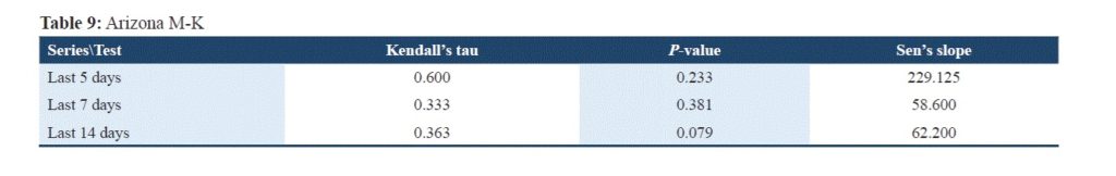
For Arizona (and Texas) data, the author ran 3 Mann-Kendall tests separately:
- $H_0$: There is no monotonic trend in the data over the last 14-day period.
$H_1$: There is a monotonic trend in the data over the last 14-day period. - $H_0$: There is no monotonic trend in the data over the last 7-day period.
$H_1$: There is a monotonic trend in the data over the last 7-day period. - $H_0$: There is no monotonic trend in the data over the last 5-day period.
$H_1$: There is a monotonic trend in the data over the last 5-day period.
The p-values for the Mann-Kendall test are all statistically insignificant.
In the prior 14-day and 7-day periods there are strong, although not significant, associations between the rates of cases and time. In the last 5-day period the association is considerably strong but remains statistically insignificant. Based on Sen’s slope, which determines the rate of change per unit time, the following remarks can be stated: in the prior 14-day period there is a 62.2 individuals/100000 individuals increase in average daily which is approximately equal to the increase in the previous 7-day period; in the last 5-day period the change in the rates of cases per unit time quadruples the increase that occurred in the above-mentioned periods.
The findings of the Mann-Kendall tests Kendall correlation coefficients and Sen’s slopes for the Texas data confirm the findings of Mann-Whitney tests and Spearman’s correlations exclusively for these data. It can be noticed that Kendall’s correlation coefficients are incrementally increasing in the prior 14-day, 7-day and 5-day periods, they all are between moderate to strong numbers in magnitude. However, the statistically insignificant values for the Mann-Kendall test do not allow to conclude that the data are increasingly plotted over time. Sen’s slopes indicate that there is a 41 additional units change in average daily in the prior 14-day period, which doubled in the prior 7-day and tripled in the prior 5-day periods. So, the additional rates of cases per unit time in average increase considerably over time, but since M-K tests null hypothesis could not be rejected, an increasing trend cannot be asserted.
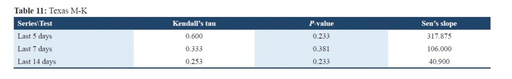
Table 10
Mann-Kendall tests and Kendall’s correlations for the Louisiana data over various time periods
For Louisiana data, Kendall’s correlation coefficients are doubled related to its precedent over the past 14-day, 7-day and 5-day periods. The increase in the average change per unit time of the rates of cases, determined by Sen’s slopes, is remarkably high in magnitude. The percent change per time unit between the examined time intervals is given below:
| 14-day and 7-day | 7-day and 5-day | 14-day and 5-day |
| 860 | 153.82083 | 2336.68 |
Although the Mann-Kendal tests findings are statistically insignificant and in agreement with Mann Whitney findings, the correlation coefficients and magnitude of slopes give the impression of strong average increases per unit time.
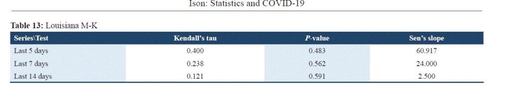
Table 11
Mann-Kendall tests and Kendall’s correlations for the Georgia data over various time periods
Similar patterns are followed for Georgia where the percent increase over the previous periods are
| 14-day and 7-day | 7-day and 5-day | 14-day and 5-day |
| 95.41083 | 327.74106 | 735.85234 |
The Georgia data lead to same observations as the Louisiana data.
The remarkably interesting result here is that, although it had been reported that they were surges in cases in Louisiana, the examination of the data does not support such statements.
Conclusions
The vast majority of the non-parametric statistical tests used are all similar, but many of them must be conducted in order to determine common findings.
They all help in identifying trends in the data, evaluating their magnitudes, and avoiding fallacies due to examination of everyday reports.