Author Notes

Data collection, design of analysis and methodology were found in a 2014 published paper:

Explanation of the mechanical example

The micro-electrical discharge machining (micro-EDM) is a non-conventional machining process which utilizes electro-thermal, non-contact effects to remove material from the workpiece by means of electric spark erosion. The metal removal process is performed by applying a pulsating (pulse on-off) electrical charge of high frequency current through the electrode to the workpiece. Both electrode and workpiece are immerged in a solution and some machining and system factors (time of the process, peak current, voltage, flushing pressure exerted on the liquid, capacitance, etc.) affect the micro-EDM performance which is measured in terms of material removal rate, and/or surface roughness, and /or tool wear rate etc.

In this experiment, the researchers decided to investigate the influence of four input factors namely, peak current, pulse on time, gap voltage, and flushing pressure on performance factor material removal rate, $MRR$.  They set some values for each factor, and based on a central composite  design, they performed 31 experimental trials. In each trial, $MRR$ was measured by calculating the difference in weight of the work piece before and after machining per time unit.

In statistical terms, the independent variables of this experiment are pulse on time, peak current, gap voltage, and flushing pressure denoted by:

• time (measured in μs),
• current (measured in A),
• voltage (measured in V),
• flspress (measured in kg/cm² )

and the dependent variable is

• material removal rate, $MRR$ (measured in mg/min)

The measurements of the experiment are imported from the article’s excel file:

Table 1

 Original Data of The Experiment

	time (μs)	current (A)	voltage (V)	flspress (kg/cm2)	$MRR$ (mg/min)
1	8	1.5	40	0.25	0.042222
2	1	1.5	40	0.25	0.025579
3	4	2	35	0.2	0.049035
4	12	1	35	0.2	0.025431
5	4	1	45	0.3	0.011455
6	12	2	45	0.3	0.029174
7	8	1.5	40	0.25	0.045261
8	4	2	45	0.2	0.066706
9	8	1.5	40	0.35	0.060853
10	8	1.5	40	0.15	0.076863
11	8	2.5	40	0.25	0.023858
12	8	1.5	40	0.25	0.043277
13	12	1	45	0.3	0.024197
14	4	1	35	0.3	0.048875
15	16	2	45	0.3	0.03
16	8	1.5	40	0.25	0.04468
17	8	1.5	40	0.25	0.040844
18	12	2	35	0.2	0.029243
19	12	2	35	0.2	0.045329
20	8	0.5	40	0.25	0.002098
21	8	1.5	30	0.25	0.042817
22	4	1	45	0.2	0.00879
23	4	2	35	0.3	0.017848
24	4	2	45	0.3	0.015584
25	8	1.5	50	0.25	0.024866
26	12	1	35	0.3	0.06402
27	12	2	45	0.2	0.072514
28	8	1.5	40	0.25	0.045852
29	8	1.5	40	0.25	0.043211
30	12	1	45	0.2	0.012752
31	4	1	35	0.2	0.021231

The set of data will be called $datat$

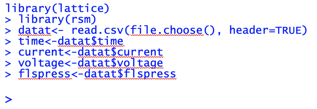
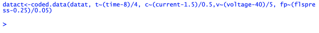
It is recommended to codify the data and perform the analysis with coded data rather than the original one (more explanations in the following pages). The codification is made by using a simple standardization-like transformation:

Variables	Transformation
time	t=(time-8)/4
current	c=(current-1.5)/0.5
voltage	v=(voltage-40)/5
flspress	fp=(flspress-0.25)/0.05

The coded variables time, current, voltage and flspress will be denoted by:

• $t$
• $c$
• $v$
• $fp$

and their set will be called datact.

Are the multilinear regression models that are developed based on the coded and the un-coded data the same?

No, the models are not the same, however, they convey exactly the same information. The regression coefficients are not the same, but the residuals, the coefficients of determination, and the F test statistics are the same.

Let us consider the following two multiple regression models: $model1.rsm$ based on the original data and $model2.rsm$ based on the coded data.

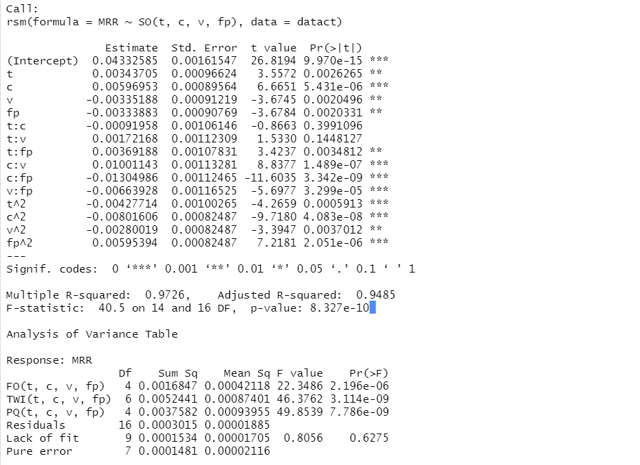
Figure 1

The Summaries of the Multi-Regression Models Based on the Original (A) and the Coded (B) Data

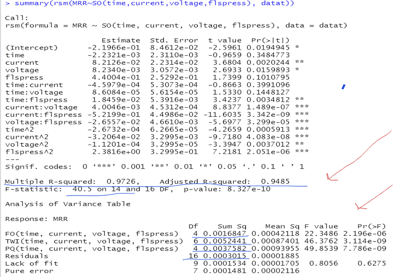
This R-output describes the multi-regression model based on the un-coded, original data. The coefficient of determination is equal to 97.26%, the adjusted coefficient of determination is equal to 94.85% . The residuals variance, in the $Mean\ Sq\ for\ Residuals$ column, is equal to 0.00001885, with 16 degrees of freedom (number of observations minus number of estimated coefficients in the model: 31-15=16)

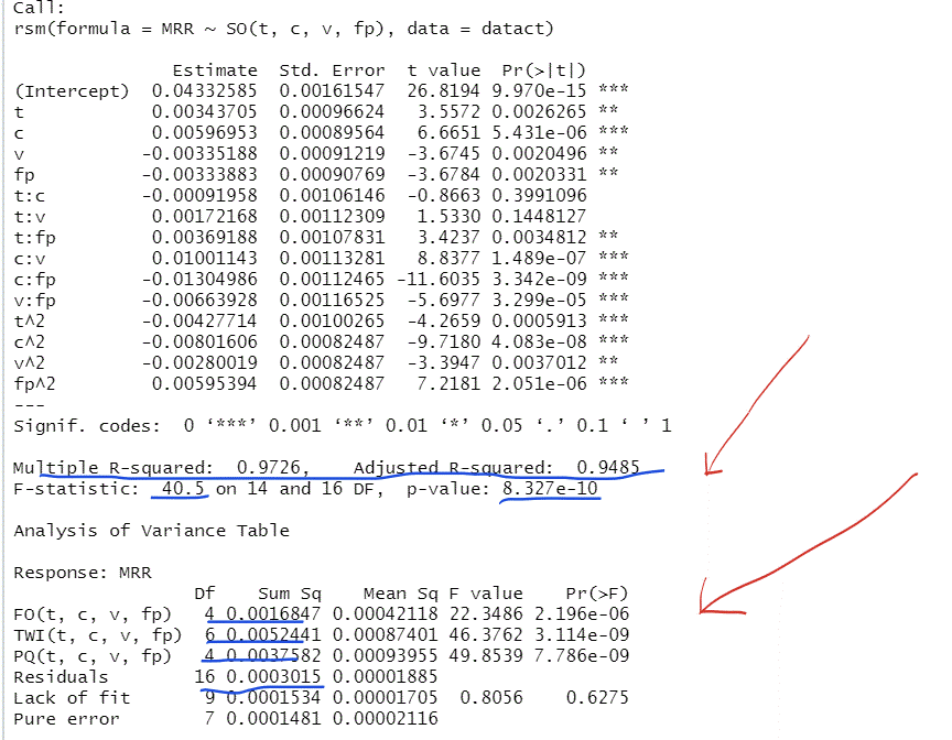
This R-output gives the multi-regression model based on the coded, transformed data. The coefficient of determination is equal to 97.26%, the adjusted coefficient of determination is equal to 94.85% . The variance of the residuals is equal to 0.0000185 with 16 degrees of freedom.

The F statistic is the same number in both models.

In conclusion, although the regression coefficients in the models are not the same, the statistics that reveal the behavior of the data and consequently the information obtained by each model remain unchangeable.

Suppose there are two multivariate regression models that are based on the same experimental data, but the output variable measurements are given in different units of measurement. Are they the same?

The authors of the article in another common work, which will be called article (B),

used the same input data, experimental settings, and output variables, but the output variables were measured in different units of measurement: in the currently studied experiment, $MRR$ was measured in mg/min, although in article (B ) in μg/min. So, the $MRR$ measurements of the second article are the $MRR$ measurements of the first multiplied by the conversion factor 1000. We call the data set of the article (B)’s experiment datactb . Then, we will work with two multiple regression models: the model associated with the first article’s experiment based on the codified data datact and noted as $model2.rsm$, and the model of article (B)’s experiment based on the codified data datactb which will be noted as $model4.rsm$:

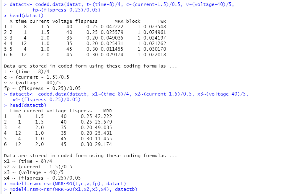
Figure 2

R-Outputs for $model2.rsm$ and $model4.rsm$

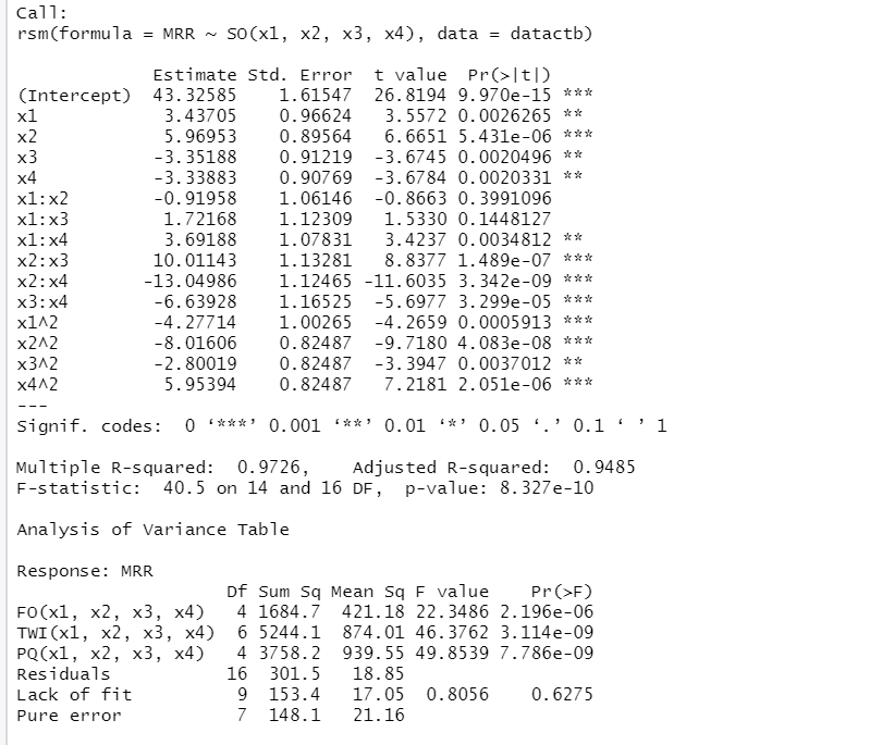
So, from the R-outputs we obtain the explicit equation of the models and much more information:

$model2.rsm:$

$MRR\ =0.0433+0.0034\ast t+0.006\ast c-0.0034\ast v-0.0033\ast fp-0.0009\ast t\ast c$

$$+0.0017\ast t\ast v+0.0037\ast t\ast fp+0.01\ast c\ast v-0.013\ast c\ast fp-0.0066$$

$$\ast v\ast fp-0.0043\ast t^2-0.0080\ast c^2-0.0028\ast v^2+0.006\ast{fp}^2$$

$model4.rsm:$

$MRR=43.3259+3.4371\ast x1+5.9695\ast x2-3.3519\ast x3-3.3388\ast x4-0.9196$

$$\ast x1\ast x2+1.7217\ast x1\ast x3+3.6919\ast x1\ast x4+10.0114\ast x2\ast x3$$

$$-13.0499\ast x2\ast x4-6.6393\ast x3\ast x4-4.2771\ast{(x1}^{)2}-8.0161\ast\left(x2\right)^2$$

$$-2.8002\ast({x3)}^2+5.9539\ast({x4)}^2$$

The regression estimates and fitted values of $model2.rsm$ scale the estimates of regression coefficients and the fitted values of $model4.rsm$ by the conversion factor 1000 (Figures 2 and 3).

Figure 3

The Actual and Fitted Values Based on $model2.rsm$ (First and Third Column) and $model4.rsm$ (Second and Fourth Column)

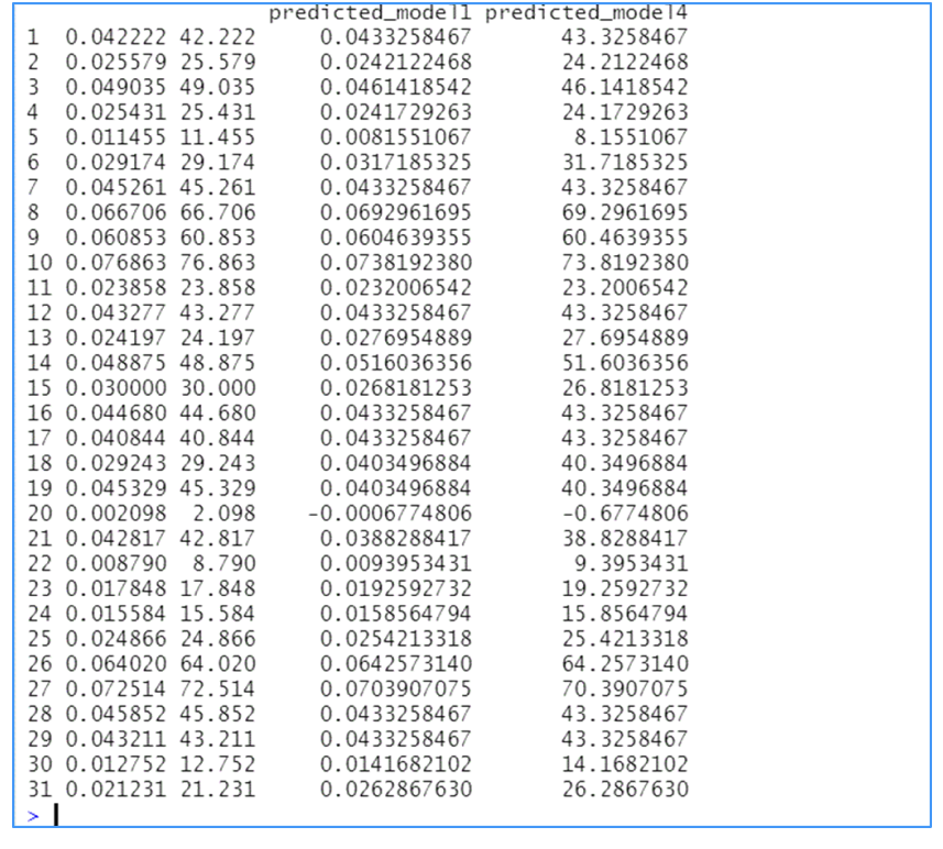
At a first glance, the regression coefficients are not similar, but a more thorough examination shows that the coefficients of the independent variables in $model4.rsm$ are the corresponding coefficients in $model2.rsm$ multiplied by the conversion factor 1000. The conclusions deduced by the regression analysis are the same because the coefficients of determination, the F test statistics associated with each one of the models are equal. The residual standard error, the sequential sum of squares, the sum of residuals, the sum of squared regression of the model based on observations measured in mg/min are the corresponding quantities of the model based on observations measured in (μg/min) multiplied by the units conversion factor or some of its powers (Table 2)

Table 2

Comparison Between the Statistics Associated with the Two Models

	$model2.rsm$	$model4.rsm$
Coefficient of determination	97.26%	97.26%
Adjusted coefficient of determination	94.85%	94.85%
Overall F test statistic	40.5 on 14 and 16 degrees  of freedom	40.5 on 14 and 16 degrees  of freedom
Residual standard error	0.004341 on 16 degrees of freedom	4.341 on 16 degrees of freedom
Sequential sums of the first order	0.0016847	1684.7
Sequential sums with interactions	0.005244	5244
Sequential sums of the second order	0.003758	3758
Residuals	0.0003015	301.5

Simple mathematical operations explain the transformation of coefficients.

What is the lack of fit?

The lack of fit is a test used to assess the quality of the fitted model. This test can be performed ONLY if there are replications in the data, otherwise the test is meaningless.

The lack of fit test examines the null hypothesis:

$H_0$: The model fit the data well, i.e., there is no need to check models with variables of higher order.

So, if the lack of fit test  is statistically significant, then the next higher power model must be examined, because it means that the model does not fit the data well and new variables must be introduced in the model.

If the lack of fit test does not give statistically significant results (so the current model is not worse than the next higher order model), we do not continue the research for a better model.

When the lack of fit is applied, the sum of squared errors, i.e., the sum of the squared residuals, is divided into two parts: one part is the sum of squared errors (deviations) due to replications (pure error) and the other the sum of squared errors attributed entirely to the model:

$SSE$ = $SSE$(lack of fit) + $SSE$(pure error)

Computation of the SSE(pure error), i.e., errors due to the replications

We group together the replications for which the experimental settings are the same. The response variable takes on unequal values for each of these trials and in that way pure error, i.e., error caused by the measurements, is created. In our experiment, we do have repeated observations.

Firstly, 7 observations with the same values for $t, c, v, fp$ and different values for $MRR$:

Table 3

Replications of the Predictors $t, c, v, fp$ at the Setting (0,0,0,0)

# of trial	t	c	v	fp	MMR
1	0	0	0	0	0.042222
7	0	0	0	0	0.045261
12	0	0	0	0	0.043277
16	0	0	0	0	0.04468
17	0	0	0	0	0.040844
28	0	0	0	0	0.045852
29	0	0	0	0	0.043211

For all the above observations the variable $t$ is set at 0 (which is the un-coded value 8 μs) and the same for the variables $c, v, fp$. The experimental measurements of the output variable in every trail are described in the last column of Table 3.The mean value of the above 7 measurements of $MRR$ is

$$(0.042222+0.045261+\ldots0.043211)/7\ =\ 0.043115$$

Then, to estimate the variability of each individual $MRR$ value about the mean of replicated observations, we compute the sum of squared distances of these values from the mean:

$${(0.042222-0.043115)}^2+{(0.045261-0.043115)}^2+\ldots+\left(0.04468-0.043115\right)^2=$$ $$=2.06423\ast{10}^{-5}$$

Another set of replicated observations is at the setting (-1,-1,-1,-1):

Table 4

Replications of the Predictors $t, c, v, fp$ at the Setting (-1,-1,-1,-1)

# of trial	$time$	$current$	$voltage$	$flspress$	$MRR$
18	1	1	-1	1	0.029243
19	1	1	-1	1	0.045329

The average $MRR$ of the two measurements is 0.037286 and similarly, their deviations about the mean is

$${(0.029243-0.037286)}^2+{(0.045329-0.037286)}^2=0.00012938$$

The mean square of the sum of squared errors due to the pure error, $(MSE(Pure\ Error))$, is defined as the pooled variance of replications and, according to the definition of the variance, is equal to the sum of the squared deviations from the mean divided by the number of replications decreased by one unit for each group of replications:

$$MSE\left(Pure\ Error\right)=\frac{2.06423\ast{10}^{-5}+0.00012938}{\left(7-1\right)+(2-1)}=\frac{0.00015}{6+1}=0.00015/7=0.00002116$$

Consequently, the variation due to the pure error, i.e., the variation that depends on the measurements is 0.00002116.

The lack of fit is the rest of the variation of the errors, which does not depend on the measurements. The sum of squared errors, the squared differences between actual values and predictions, is equal to 0.0003015 and represents a measure of the errors:

$$Sum\ of\ Squared\ Errors\ of\ Lack\ of\ Fit\ =\ 0.0003015-0.00015=0.0001534$$

The degrees of freedom of errors due to the of lack of fit is the difference between the degrees of freedom of errors (residuals) and the degrees of freedom of errors of pure error, according to the equation SSE = SSE(lack of fit) + SSE(pure error). Consequently,

$$Degrees\ of\ freedom\ Errors\ due\ to\ the\ Lack\ of\ Fit\ =\ 16-7=9$$

According to the definition of the variance, the variance of the errors caused by the lack of fit, i.e., the mean square of the SSE(lack of fit), is the ratio of the sum of squared errors of lack of fit divided by the degrees of freedom of errors due to the lack of fit:

$$Mean\ Square\ of\ the\ SSE\left(Lack\ of\ Fit\right)=$$

$$=\frac{Sum\ of\ Squared\ Errors\ of\ Lack\ of\ Fit\ }{Degrees\ of\ freedom\ of\ Sum\ Squared\ Errors\ of\ Lack\ of\ Fit}=\frac{0.0001534}{9}$$

Intuitively, it is understood that the test statistic of the lack of fit must be a number that compares the variance due to the measurement errors against the variance due exclusively to the model.

So, the sum of squared errors due to the lack of fit and specifically its variance (i.e., the mean square of the sum of squared errors due to the lack of fit) must be compared to the variance of the sum of squared errors due to the pure error (i.e., the mean square of the pure error). Therefore,

$F=\frac{MSE\left(Lack\ of\ Fit\right)}{MSE\left(Pure\ Error\right)}$ $=\frac{0.0001705}{0.00002116}=0.8056$

A lack of fit mean square that is considerably larger compared to the pure error mean square suggests that the model does not fit the data well.

In contrast, in the experiment studied, the lack of fit mean square is nor considerably greater than the pure error mean square, so the F-test is not statistically significant and there is no evidence to reject the null hypothesis $H_0$. Consequently, there is no lack of fit and the model fits the data well.

In conclusion, with the above-mentioned lack of fit F-test there is a thorough examination about how well the chosen model fits the data.

Is the sum of squared errors of pure error associated with the model?

No.

The pure error is independent of the model. Obviously, the pure error depends on the values of the output variable at the replicated observations. For the computation of the variation due to the pure error we used the number and magnitude of replications. The characteristics of the model namely, its order and its number of estimated coefficients, did not interfere with any of the above calculations.

Is it possible to perform the lack of fit test when there are replicated observations (several measurements at the same input variables) with equal values of the output variable at each of these settings?

No, because the sum of squared errors of lack of fit is the sum of squared errors minus the sum of squared errors of pure error, and the pure error can be computed only if there are replicated observations at which the output variable takes on unequal values. Let us consider another work,

where the same mechanical experiment is studied with input variables capacitance ($pF$) voltage ($V$) and tool rotation speed ($rpm$) and output variable the crater.size. The data imported from the article are called datapj and the regression model is $modelpj.rsm$:

Table 5

 Original and Coded Data of the Experiment Based on datapj Data

c	v	tr	capacitance	voltage	tool_rotation	Crater. size
-1	-1	0	30	60	2000	0.45
1	-1	0	4700	60	2000	11.2033
-1	1	0	30	110	2000	1.854
1	1	0	4700	110	2000	12.69
-1	0	-1	30	85	1000	0.821
1	0	-1	4700	85	1000	8.46
-1	0	1	30	85	3000	2.1014
1	0	1	4700	85	3000	8.46
0	-1	-1	1000	60	1000	4.13
0	1	-1	1000	110	1000	5.84
0	-1	1	1000	60	3000	4.256
0	1	1	1000	110	3000	7.192
0	0	0	1000	85	2000	5.88
0	0	0	1000	85	2000	5.88
0	0	0	1000	85	2000	5.88

The data were coded under the transformations:

Variables	Transformation
capacitance	$c$=(capacitance-1000)/3700
voltage	$v$=(voltage-60)/25
tool rotation	$tr$=(tool rotation-2000)/1000

Figure 4

R-Output for the Model of the Second Order Based on $Datapj$

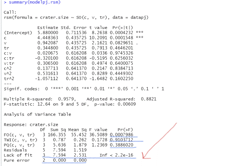
The second order model is

$$crater.size=5.88+4.448\ast c+0.942\ast v+0.3448\ast tr+0.0207\ast c\ast v-0.32\ast c$$

$$\ast tr+0.3065\ast v\ast tr+0.1377\ast c^2+0.5316\ast v^2-1.057\ast{tr}^2$$

The overall F test statistic is equal to 12.64 and provides strong evidence that the model explains the data better than the baseline model (baseline is the model that suggests that none of the variation in crater.size is explained by any of the input variables and consequently its prediction values are equal to the mean of crater.size at any predictors setting).

Put it in another way, the models that has 9 variables explains the data better than a model with no variables, but  with only one intercept (i.e. the mean of crater.size ). This is expectable.

The model has many problems related to the statistical (in)-significance of both the regression coefficients and the sequential sums of squares:

together with the estimation of every regression coefficient R applies a t-test related to the coefficient checking the hypothesis:

$H_0$: the real regression coefficient for the models that refers to the whole population is zero

In other words, the above null hypothesis suggests that the estimated coefficient of the input variable occurs randomly and this coefficient in the true regression model based on the whole population is zero.

This is an interesting hypothesis since if there is not strong evidence that $H_0$ can be rejected, then the corresponding variable does not have any impact on the dependent variable, and it is redundant in the model. We immediately observe that only the intercept and the coefficient of $c$ (current) are statistically significant though the coefficients of higher order variables and their interactions are not statistically significant ($Analysis\ of\ Variance$ Table of the R-output)

Similarly, for the sequential sum of squares the following null hypothesis is investigated:

$H_0$: the current model is not better than the precedented

or formulated in different words:

$H_0$: dropping the additional variables do not harm the situation

The calculations in the R-output show that the additional interaction terms are not statistically significant. So, there is no need to add them in the model.

Apparently the same is true for the additional squared variables.

We will (wrongly) apply a lack of fit test to highlight the problem that is rising when lack of fit test applies on database where the output variable takes on the same arithmetic value for all settings of the replicated observations (Figure 4).

The lack of fit test suggests that the model does not fit the data well, so we have to create models with higher order variables, although the previous t-tests on the estimated coefficients show that there is no need of additional variables in the model other than the first order variables. Contradiction!

The misleading results of the lack of fit tests are caused by the fact that real pure error is equal to zero.

Pure error is the variance explained by the replicated observations, meaning the predictor variables take on the same set of values, but the output variable gets on a new value at each experimental setting. In contrast, in this experiment the crater.size values at the three experimental settings are all equal (the last three observations).

The mean value of crater.size of the replicated observations is (5.88+5.88+5.88)/3 =5.88.

By definition, degrees of freedom must be assigned to the pure error, specifically 3-1=2 since there are three replicated observations, but the sum of squared errors of the pure error is (obviously) zero:

$$SSE\left(Pure\ Error\right)=\ {(5.88-5.88)}^2+{(5.88-5.88)}^2+{(5.88-5.88)}^2=0$$

So, for calculating the F ratio, the division $F=\frac{2.531}{?}$ is unacceptable, and the result becomes misleading

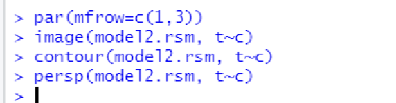
Graphical visualization of the response surface

After studying the fitted model, a graphical visualization of the fitted surface is presented, which is particularly useful when response surface methodology techniques are employed.

The easier way to present a fitted surface is by using some ready commands in RStudio which describe a part (portion) of the surface formed by the predicted values.

Since the fitted model contains a large number of input factors and obviously in a 3D representation only two input factors are used, we must specify the chosen variables.

It is especially important to notice that these surfaces describe graphical presentation of the predicted values in small neighborhoods and, if another remote neighborhood is chosen very probably the surface will be different.

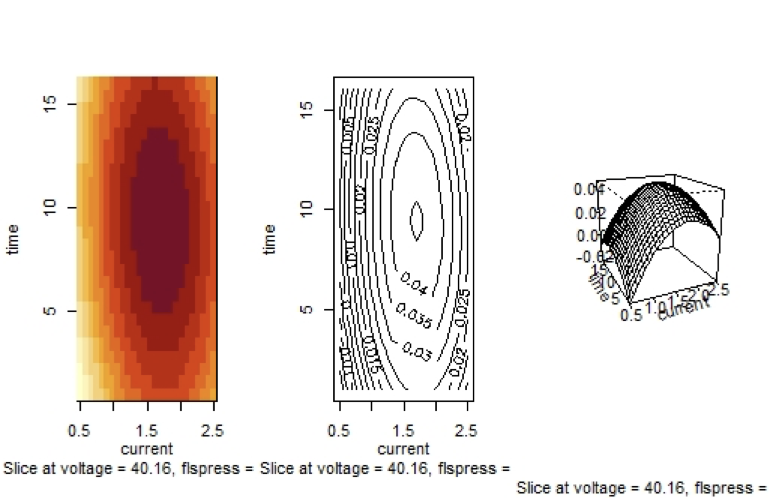
Some (portions) of the fitted surface of $MRR$ are presented below:

$MRR$ surface against $t, c$

Graph 1

Fitted Surface of $molel2.rsm$ with Independent Variables $t, c$

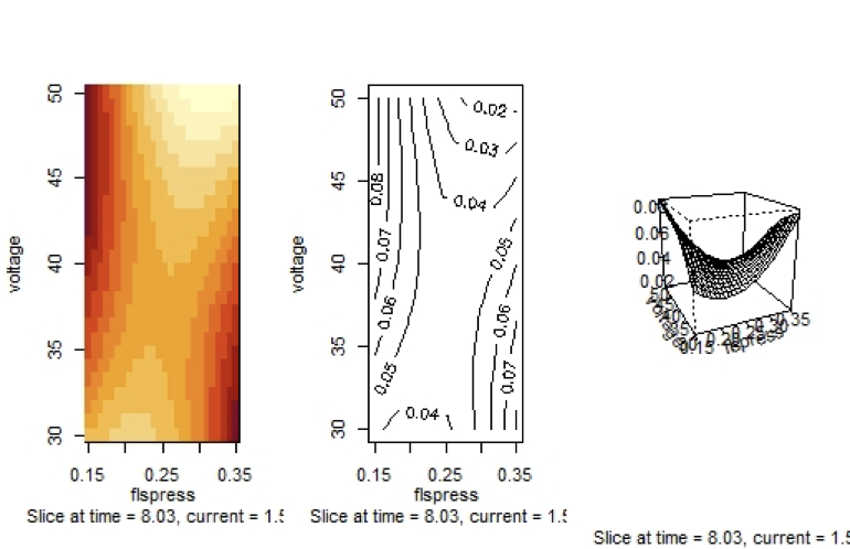
Graph 2

Fitted Surface of $molel2.rsm$ with Independent Variables $v$ and $fp$

Graph 3

Fitted Surface of $molel2.rsm$ with Independent Variables $t$ and $fp$

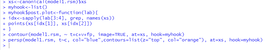
It is possible to create some codes to enhance the fitted surface:

In case of a multiple regression model the fitted surface is formed for every two independent variables while the rest of the independent variables get some fixed value, which by default  are the central values of the independent variables that do not appear in the graph. It would be more interesting to vary two independent variables while the others keep their values at the stationary point of the surface.

Then an enhanced graph of the surface is formed by determining firstly the stationary points:

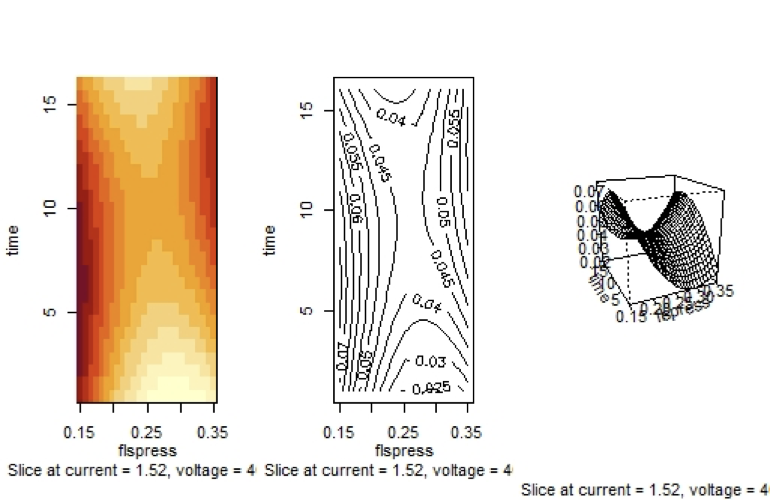
Graph 4

Contour Plots of the Output Variable MRS as Function of two of the Input Variables

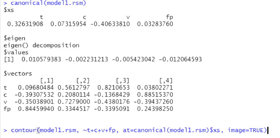
Reading the output of the command canonical() and canonical path()

A part of the summary of the rsm model provides us with the eigenvalues and their eigenvectors. The same results can be obtained by using the function canonical()

A stationary point can be either a maximum or a minimum or a saddle point ( i.e. neither maximum nor minimum). If all signs of the eigenvalues are positive then the stationary point is a minimum, if all signs of the eigenvalues are negative then the stationary point is a maximum and in case of mixed signs it is a saddle point. In the command canonical()

the at argument provides the location around which the fitted surface is located.  The at argument sets the values at which to hold independent variables, other than the ones that appear on the coordinate system. In this case, the at argument has to be set at the stationary point. If we set the argument image as true, each contour plot is a colored image overlaid by the contour lines.  Then, we obtain the same results as in the previous paragraph related to the contour plots: the contour plots of $MRR$ as function of $t$ and $c$ centered at the stationary point, or as function of two of the independent variables of the experiment.

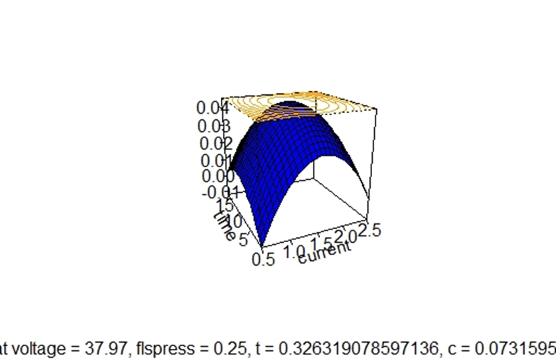
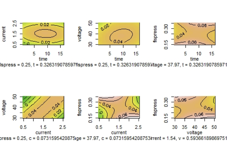
Graph 5

Contour Plots of the Output Variable MRS as Function of two of the Input Variables

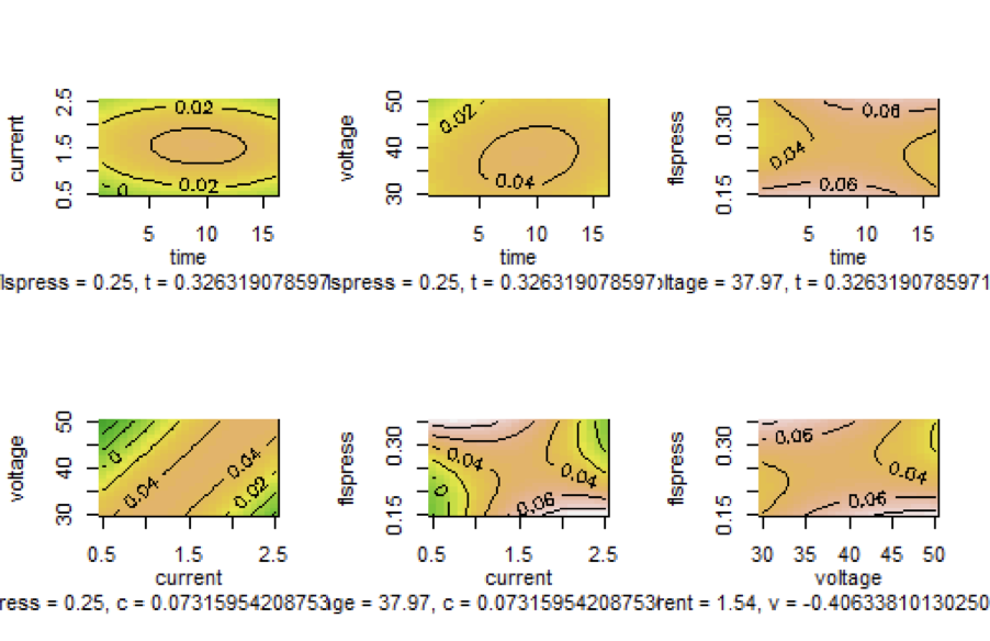
Since there are four eigenvalues one positive and three negatives, the stationary point is a saddle point which means that it is not a point at which we have an optimum value of the surface. By observing the contour plots, the nonexistence of a point at which $MRR$ has a maximum value is obvious since the maximum of the output value lies at the center of the contour lines, and in the above contours we do not have such a common internal contour. When considering $MRR$ as a function of time and current there is a central contour line at which $MRR$ takes on the value 0.02. When considering $MRR$ as a function of $t$ and v there is a central line at which $MRR$ takes on the value 0.04. In all other contours there is no central line. Indeed, the portion of surface representing $MRR$ as a function of $t$ and c has a maximum, although other surfaces representing $rsm$ as function of other input variables do not follow the same patterns.

In this case, the researchers must make some more trials: choose “good data” by marching in the direction of the saddle point and adding small increments in the independent variables, perform a new experiment and by observing the new response values of the output variable find another stationary point, hopefully maximum or minimum. This procedure can be repeated many times because the optimal point can be out of sight. If the stationary point is in the design space, it makes sense to start at the stationary point and explore the most steeply rising ridge in both directions. The command canonical.path() provides a good idea about the path to be followed, and the distance is a signed quantity according to the direction that will be followed. The canonical.path() below describes a region of radius 4.

Table

The Best Path to Be Followed for the Location of the Optimum Point, Starting at the Stationary Point

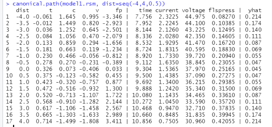
In the above calculations, all four parameters are incremented simultaneously, and the dependent variable is measured. It must be noticed that the increments are added to the coded parameters while considering the directions suggested by the stationary point.