Author Notes

Data collection, design of analysis and methodology were found in a 2018 published paper:

 Description of the experiment. Terminology

In this research study, fans specifications are examined in order to provide manufacturers with the instructions for the production of strong, more efficient, and long-lasting cool fans. Given that typical applications of fans  include, but they are not limited to, personal thermal comfort, vehicle engine cooling systems, machinery cooling systems, fume extraction, winnowing, and numerous others, their reliability is a crucial problem in fans manufacturing industry. Therefore, the process of finding the best settings from all feasible settings is an interesting statistical problem.

Three are the fan’s characteristics studied in this experiment: the type of the  hole shape in the fan blade, the shape of the hub or barrel surface into which the blade is placed, and the type of assembly method for the two components. In statistical terms, there are three independent variable $x_1, \ x_2, \ x_3$ with two levels each.

• $x_1$: Hole shape coded as hex holes (-1), or round holes (1)
• $x_2$: Shape of hub coded as knurled (-1), or smooth (1)
• $x_3$: Type of assembling method coded as staked (-1), or spun (1)

The efficiency and performance of the fan is measured by estimating the tarque force required to break the fan. So, the dependent variable is tarque force.

$y: Tarque\ force$

Matrix Equation Equivalent to a Second-Order Multiple Regression Model

The authors decided to form a second-order multiple regression model to determine the simultaneous effects of the independent variables on the dependent variable. Without going into details, which are described in previous lessons, the quadratic model based on their collected data is

$$\hat{y}=180.23+2.4029\ast x_1+1.8705\ast x_2+30.776\ast x_3-43.805\ast x_1^2-44.158{\ast x}_2^2$$

$$-21.006\ast x_3^2-2.2335\ast{10}^{-14}\ast x_1\ast x_2+1.25\ast x_1\ast x_3 -x_2\ast x_3$$

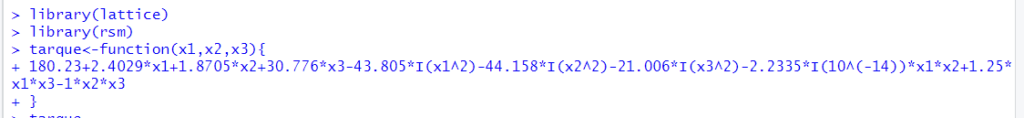
In R, it is possible to describe such a model without the use of the commands lm( ) or rsm( ), where the explicit set of data is needed, by using the command function( ) with argument $x_1, \ x_2, \ x_3$ as it is explained in Figure 1:

Figure 1

R -Commands for Fitting the  Multiple Regression Model

The second-order model is mainly used for predictive purposes, i.e., if the independent variables $x_1, \ x_2, \ x_3$ are substituted by a set of their experimental values, then a fitted (predictive) value for the dependent variable is obtained which is an estimation of the real experimental value of $y$. Consequently, the model can be used in a region near the experimental values for $x_1, \ x_2, \ x_3$ to predict the values of $y$. The coefficients of the variables $x_1, \ x_2, \ x_3$ in the right-hand side of the equation play an important role in the construction of the model and are calculated based on calculus formulas.

$$\hat{y}=b_0+\ t\left(X\right)\ast b+t\left(X\right)\ast B\ast X$$

where $b_0=180.23$, $X=\left[\begin{matrix}x_1\\ x_2\\ x_3\ \end{matrix}\right]$ , $b=\left[\begin{matrix}2.4029\\ 1.8705\\ 30.776\ \end{matrix}\right]$

$$B=\ \left[\begin{matrix}-43.805&-1.1168\ast{10}^{-14}&0.625\\ -1.1168\ast{10}^{-14}&-44.158&-0.5\\ 0.625&-0.5&-21.006\ \end{matrix}\right],$$

and t(matrix) is the transpose of the matrix, i.e.,

$t\left(b\right)=\ \left[\begin{matrix}2.4029&1.8705&30.776\ \end{matrix}\right],$ or

$$t\left(X\right)=\left[\begin{matrix}x_1&x_2&x_3\ \end{matrix}\right]$$

The row matrix $X$ is the matrix of the three independent variables${\ \ x}_1,\ x_2,x_3$ and the column matrix $b$ is the matrix of their coefficients in the second-order equation.

So, the matrix multiplication of the row matrix $X$ times the column matrix $b$ results in an element matrix, which is the sum of the first-order factors in the model.

The 3×3 matrix $B$ is the matrix of the coefficients of the second-order terms and the interaction terms of ${\ x}_1,\ x_2,x_3$ namely, $x_1^2,\ x_2^2,\ x_3^2$ and $x_1\ast x_2,\ { \ x}_1\ast x_3\ ,\ x_3\ast x_2\ $ . The element at the first row and first column is the coefficient of $x_1\ast x_1=x_1^2$ in the second-order model. Similarly, the element that lies in the first row and second column is the model coefficient of $x_1\ast x_2$ . The element at the second row and second column is the coefficient of $x_2\ast x_2=x_2^2$ . All the elements of matrix $B$ are formed following that pattern.

$B$ must satisfy two important properties in order to be consistent with the principles of matrices multiplication:

• It must be symmetric, i.e., the element at the first row and second column is equal to the element at the second raw and first column. Similarly, the element at the first row and third column is equal to the element at the third raw and first column and so on.  In general, the symmetric property of the matrix $B$ imposes the condition: $b_{ij}=b_{ji}$ , where $b_{ij}$ is the matrix element that lies in the i row and j column.
• The sum of the elements at the first row and second column plus the element at the second raw and first column is equal to the coefficient of $x_1\ast x_2$, so each of them is equal to its half, $b_{12}+b_{21}=-2.2335\ast{10}^{-14}$ . This is true for all the non-diagonal $B$ elements: $b_{ij}+b_{ji}=coefficient\ of\ x_{ij}$

The necessity of the above matrix structure is proven by making the explicit calculations:

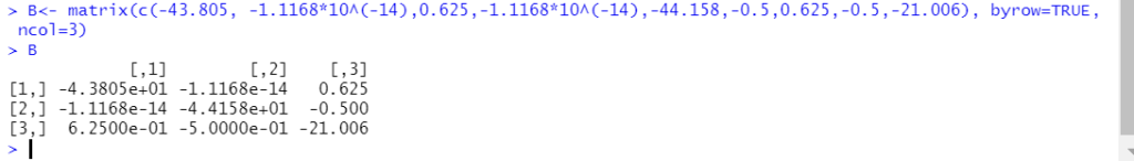
In R, the command matrix( )can generate any matrix, under the condition we specify in the argument the vector of the values that will constitute the elements of the matrix and the number of columns of the matrix. The argument “byrow=TRUE” refers to the way R has to fil the matrix, in this case by describing the rows firstly.

Figure 2

R-Commands for Setting the Matrix $B$

Stationary Points Found Using the Matrix Equation

Let $z=f(x1,x2,x3)$ be the model whose graphical presentation is a surface S. A stationary point of S is a point $x_s=(x_s1,\ x_s2,\ x_s3)$ such that the partial derivatives of $f$ with respect to $x_1,x_2,x_3$ are all equal to zero at $x_s$. It can be a local maximum or minimum or a saddle point, depending on the sign of the second partial derivatives. Instead of finding the partial derivatives of the long second-order model, it is easier to determine them by using the matrix equation:

$$\hat{y}=b_0+\ t\left(X\right)\ast b+t\left(X\right)\ast B\ast X$$

$$\frac{\partial\hat{y}}{\partial x_1}=\ \left[\begin{matrix}1&0&0\ \end{matrix}\right]\ast b+\left[\begin{matrix}1&0&0\ \end{matrix}\right]\ast B\ast X+t\left(X\right)\ast B\ast\left[\begin{matrix}1\\ 0\\ 0\ \end{matrix}\right]=$$

$$=2.4029+\left[\begin{matrix}-43.805&-1.1168\ast{10}^{-14}&0.625\ \end{matrix}\right]\ast \left[\begin{matrix}x_1\\ x_2\\ x_3\end{matrix}\right]+ \left[\begin{matrix}x_1&x_2&x_3\end{matrix}\right]$$

$$\ast\left[\begin{matrix}-43.805\\ -1.1168\ast{10}^{-14}\\ 0.625\ \end{matrix}\right]=$$

$$=2.4029-43.805\ast x_1-1.1168\ast{10}^{-14}\ast x_2+0.625\ast x_3$$

$$-43.805\ast x_1 -1.1168\ast{10}^{-14}\ast x_2+0.625\ast x_3=$$

$$=2.4029+2\ast(-43.805\ast x_1-1.1168\ast{10}^{-14}\ast x_2+0.625\ast x_3)$$

Similarly,

$$\frac{\partial\hat{y}}{\partial x_2}=\ \left[\begin{matrix}0&1&0\ \end{matrix}\right]\ast b+\left[\begin{matrix}0&1&0\ \end{matrix}\right]\ast B\ast X+t\left(X\right)\ast B\ast\left[\begin{matrix}0\\ 1\\ 0\ \end{matrix}\right]=$$

$$=1.8705+\left[\begin{matrix}-1.1168\ast{10}^{-14}&-44.158&-0.5\ \end{matrix}\right]\ast\left[\begin{matrix}x_1\\ x_2\\ x_3\ \end{matrix}\right]+\left[\begin{matrix}x_1&x_2&x_3\ \end{matrix}\right]$$

$$\ast\left[\begin{matrix}-1.1168\ast{10}^{-14}\\ -44.158\\ -0.5\ \end{matrix}\right]=$$

$$=1.8705-1.1168\ast{10}^{-14}\ast x_1-44.158\ast x_2-0.5\ast x_3$$

$$-1.1168\ast{10}^{-14}\ast x_1-44.158\ast x_2-0.5\ast x_3=$$

$$1.8705+2\ast(-1.1168\ast{10}^{-14}\ast x_1-44.158\ast x_2-0.5\ast x_3)$$

And,

$$\frac{\partial\hat{y}}{\partial x_3}=\ \left[\begin{matrix}0&0&1\ \end{matrix}\right]\ast b+\left[\begin{matrix}0&0&1\ \end{matrix}\right]\ast B\ast X+t\left(X\right)\ast B\ast\left[\begin{matrix}0\\ 0\\ 1\ \end{matrix}\right]=$$

$$=30.776+\left[\begin{matrix}0.625&-0.5&-21.006\ \end{matrix}\right]\ast\left[\begin{matrix}x_1\\ x_2\\ x_3\ \end{matrix}\right]+\left[\begin{matrix}x_1&x_2&x_3\ \end{matrix}\right]\ast\left[\begin{matrix}0.625\\ -0.5\\ -21.006\ \end{matrix}\right]=$$

$$=30.776+0.625\ast x_1-0.5\ast x_2-21.006\ast x_3+0.625\ast x_1-0.5\ast x_2-21\ast x_3$$

$$=30.776+2\ast(0.625\ast x_1-0.5\ast x_2-21.006\ast x_3)$$

Then, if we set all three partial derivatives equal to zero, we locate the stationary point $x_s$ :

$$\frac{\partial\hat{y}}{\partial x_1}=\ \ 2.4029+2\ast(-43.805\ast x_1-1.1168\ast{10}^{-14}\ast x_2+0.625\ast x_3)=0$$

$$\frac{\partial\hat{y}}{\partial x_2}=1.8705+2\ast\left(-1.1168\ast{10}^{-14}\ast x_1-44.158\ast x_2-0.5\ast x_3\right)=0$$

$$\frac{\partial\hat{y}}{\partial x_3}=30.776+2\ast(0.625\ast x_1-0.5\ast x_2-21.006\ast x_3)=0$$

The three last equations are equivalent to the matrix equation:

$$b+2\ast B\ast \left[\begin{matrix}x_1\\ x_2\\ x_3\ \end{matrix}\right]=0$$

Then, if the vector $x_s=\left[\begin{matrix}x_s1\\ x_s2\\ x_s3\ \end{matrix}\right]$ is the solution of the above matrix equation, it must satisfy:

$$\left[\begin{matrix}x_s1\\ x_s2\\ x_s3\ \end{matrix}\right]=\ -\ \frac{1}{2}\ast B^{-1}\ast b$$

Substituting the values of $x_s$ in the matrix equation of the model,

$$\ b_0+\ t\left(X\right)\ast b+t\left(X\right)\ast B\ast X$$

we have the estimated response ${\hat{y}}_s$ of the dependent variable, tarque force, at the stationary point.

As soon as the theoretical part is set, we can order R to perform the calculations:

Figure 3

R Computes the Stationary Point

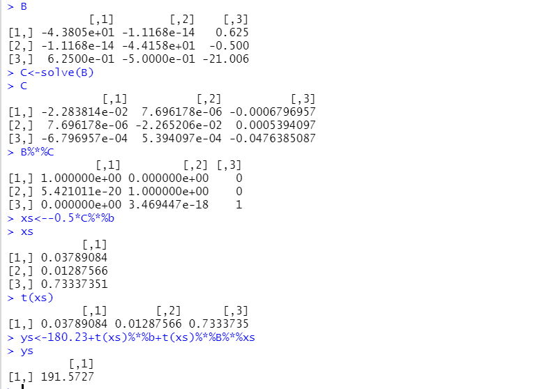
R calculates the inverse matrix of $B$ by executing the command solve$(B)$. When multiplying the two matrices, $B$ and its inverse, which will be called $C$, we get the identity matrix according to the definition (in the software program some of the non-diagonal numbers are not exactly zero because R rounds off decimals and with long decimals we have estimations of the operations). Then, by making the matrix multiplication

$$\left[\begin{matrix}x_s1\\ x_s2\\ x_s3\ \end{matrix}\right]=\ -\ \frac{1}{2}\ast B^{-1}\ast b$$

we get a column matrix of the coordinates of the stationary point:

$x_s=$ (0.03789, 0.0129, 0.7334) and $\hat{y}_s=$ 191.5727 the estimated tarque force value at $x_s$

Canonical Analysis: Translation and Rotation of the Axis with the Help of Eigenvalues and Eigenvectors

Some important features of a square matrix are its eigenvectors and eigenvalues.

For a square matrix $B$, a number lambda, λ is called an eigenvalue of $B$ if there exists a nonzero vector $v$ for which we have:

$$B\ast v=\lambda\ast v.$$

In this case $v$ is an eigenvector of the matrix $B$ belonging to λ.

Thus, an eigenvector has a strong property: When an eigenvector is multiplied by its matrix the result is a vector which is a multiple of this eigenvector; the scale factor in this case is the eigenvalue. The eigenvectors play an important role in the choice of the coordinate axis of the system and consequently in the graphical presentation of surfaces, as it is explained below.

In our example, the matrix B has three distinct eigenvectors, that can be found by performing the matrices multiplications and solving a 3×3 system.

By executing the command eigen(matrix), R performs the operations and solves the system. In this case the command order will be used as well, in order to obtain a permutation of the eigenvalues in decreasing order, in absolute value. Then, a rearrangement of the corresponding eigenvectors is requested.

Figure 4

R Provides the Readers with the Eigenvectors and Eigenvalues of B

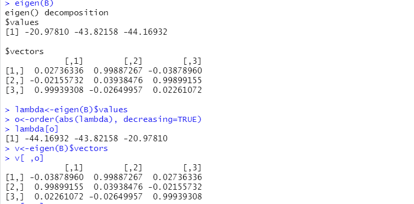
The square matrix whose columns are the eigenvector of matrix $B$, is denoted, as in the R output, as $V$; its transpose matrix is $t(V)$ .

Some particularly important theorems of Linear Algebra assure the following:

2. Theorem of diagonalization of a matrix
If a matrix of real elements has three linearly independent eigenvectors belonging to three distinct eigenvalues, which necessarily form a basis of the real space, like the matrix B in our example, then the matrix is diagonalizable, i.e., $V^{-1}$ *B*V is a diagonal matrix. The three nonzero diagonal elements of the diagonal matrix are the three eigenvalues of B.

Figure 5

Proof of the Theorem of Diagonalization  With R

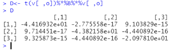
The above matrix is a diagonal one and the elements in the main diagonal are the eigenvalues, the lambda values of the example. We observe that the non-diagonal elements are digital numbers having the first non-zero digit 15, or 16, or 17 places to the right of the digital point, respectively. So, the non-diagonal elements all are practically equal to zero.

3. Theorem of the translation and rotation of the axis
By making a translation of the axis in order to get as origin the stationary point, the matrix model of the second-order equation, $\hat{y}=b_0+\ t\left(X\right)\ast b+t\left(X\right)\ast B\ast X$ , is

$$\hat{y}=b_0+\ t\left(X+xs\right)\ast b+t\left(X+xs\right)\ast B\ast\left(X+xs\right)$$

The operations between matrices and the column vector of the coordinates of the stationary  point leads to:

$${\hat{y}}_s+t\left(X\right)\ast B\ast X$$

with ${\hat{y}}_s$ the fitted value at the stationary point.

Now, if we consider as a new basis the basis of the eigenvectors and take into consideration the first theorem we have:

$$\hat{y}={\hat{y}}_s+\lambda_1\ast w_1^2+\lambda_2\ast w_2+\lambda_3\ast w_3$$

The above equation explains something especially useful: Near the stationary point the values of the fitted value $\hat{y}$ depend on the sign of the eigenvalues:

• If the eigenvalues are all negative, then the stationary point is a maximum because the fitted $\hat{y}$ ’s will be equal to $y_s$ diminished by a positive number. So, the fitted values will be smaller than the fitted value at the stationary point.
• If the eigenvalues are all positive, then the stationary point is a minimum because the fitted $\hat{y}$ ’s will be equal to $y_s$ augmented by a positive number. So, the fitted values will be greater than the fitted value at the stationary point.
• If there are positive and negative values a decision cannot be made.

Since all eigenvalues are negative, the stationary point is a MAXIMUM

Graphical Presentation

In order to visualize the surface which is the graphical presentation of the second- order model near the stationary point then we must choose as origin of the axis the stationary point and a new basis, the basis of the eigenvectors.

An important fact here is the use of Linear Algebra’ s theorems which assures that the eigenvectors form a basis, something that cannot be deduced by using R only.

In the R commands, the new coordinate plane system is introduced with horizontal and vertical axis two of the eigenvectors.

Figure 6

R-Commands for the Graphical Presentation of the Response Surface on a Coordinate System with Origin the Stationary Point and Axis the Eigenvectors V[ ,1] and V[ ,3]

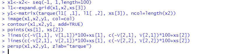
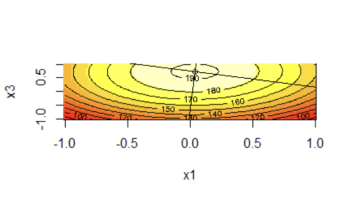
Graph 1

2D Contour Plot of  vs  and

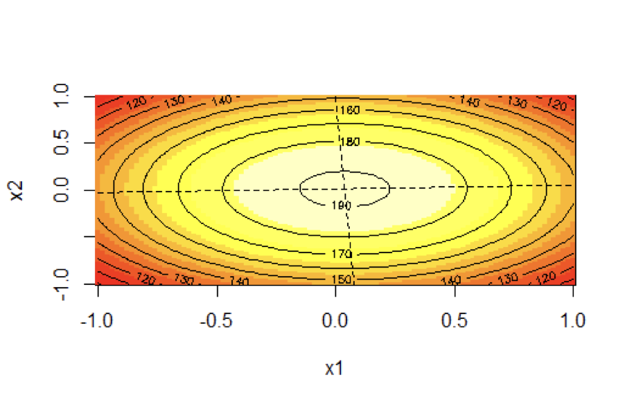
In Graph 1, the origin of the coordinate system is the point (0.03790, 0.01288) at the level of contour with $x_3$ equal to 0.7334. By observing the 2D contour plot we understand that the values of tarque force are decreasing as the points get away from the origin: The first contour line is at a value of tarque equal to 190 and then the next closest to it corresponds to a tarque force equal to 180. The values of the dependent variable are decreasing as the point get away from the origin.

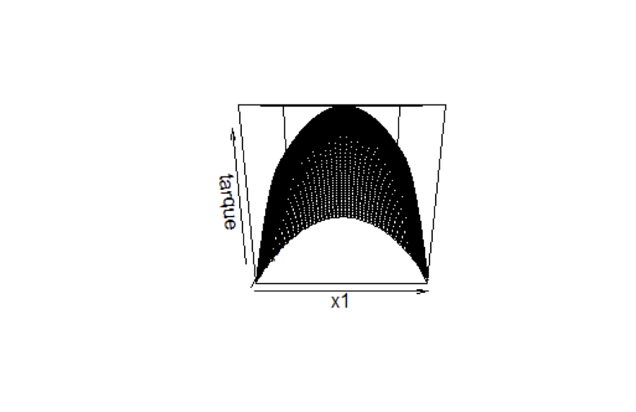
With the command persp the response surface in space is presented, but the coordinate system is the axis $x_1$ and $x_2$. We observe that the surface gets a pick.

 Graph 2

Response Surface Plot of y vs $x_1$ and $x_2$

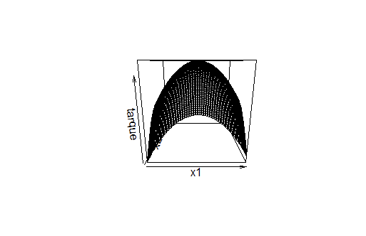
Figure 7

R-Commands for The Graphical Presentation of the Surface Y on a Coordinate System with Origin the Stationary Point and axis the Eigenvectors V[ ,1] and V[ ,3]

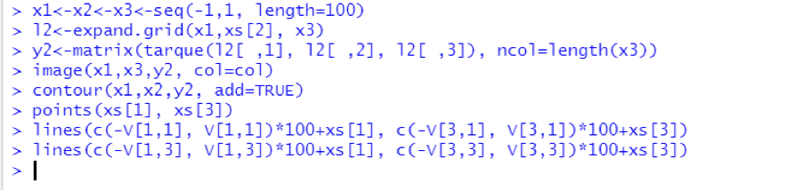
Graph 3

Contour Plot of y vs $x_1$ and $x_2$

Graph 4

Response Surface Plot of y vs $x_1$ and $x_3$