Chi-square Test

Do first born children have more self-control and self-esteem? Are middle children carefree, charming, and manipulative? Are political results influenced by the order in which candidates are listed on the ballot, with the ones whose names appear early on the list being more advantageous than those listed later? Are the same proportion of people supporting a number of different political parties? Are African Americans who murder whites disproportionally sentenced to death? These are kind of research questions that can be examined by applying the chi-square test, which, in contrast to the ANOVA tests, examines differences among categorical variables.

It is used in the following situations:

• When the categorical data can be clearly divided into mutually exclusive categories, i.e., there are no common points in any two of these categories, and it is requested to compare the observed number of data in each category with the expected number that would fall in the category if a hypothesis were true. Usually, we hypothesize that the data are coming from a theoretical well-determined distribution and check if the observed data frequencies are compatible with the theoretical frequencies.
• When the data have been categorized in two different ways, for example, by gender and propensity to commit a suicide, and it is requested to examine the independence of classification.

Chi-square test is frequently mistaken with binomial test (more details below)

Terminology

When dealing with distributions, R uses the following notations:

$ddistribution(..,..)$ density function of a distribution, for example, $dpois(x,\ lambda=\lambda..)$ denotes the density function of a Poisson distribution with parameter $\lambda$.

$pdistribution(\ number,\ parameters)$ gives the probability that a random variable X that follows a specific distribution takes on values less than or equal to the number that appears in the first place of the argument. Thus, $pnorm(85,\ 72,\ 15.2)$ is the probability that a random variable X that follows a normal distribution with mean equal to 72 and standard deviation 15.2 takes on values less than or equal to 85, although $pnorm(85,\ 72,\ 15.2,\ lower.tail=F)$ is the probability that the random variable X takes on values higher than 85.

$qdistribution(a%,parameters)$ gives the number on the x -axis of a specific distribution to the left of which there are a% of the distribution. Thus, $qnorm(0.95,\ 0,1)$ is the number on the x-axis of a standard normal distribution (the mean is equal to 0 and the standard deviation is equal to 1) to the left of which there are 95% of the distribution.

Goodness-of-fit test: 1-way classification

In this case, researchers want to estimate how similar an observed distribution is to an expected distribution.

So, for each event of the experiment there are two kinds of probabilities:

the (empirical) probabilities of the events that are calculated based on the frequencies obtained by observation

and

the expected probabilities of the events that are calculated based on the theoretical(expected) distribution of the data, as this distribution is stated in the null hypothesis.

 When applying the -test the formulation of the null hypothesis is fixed: The null hypothesis of a chi-square test always states that the data follow a theoretical distribution.

The simplest case is when the observed distribution has to be compared to the uniform distribution, i.e., the expected probabilities of all the events are equal.

For example:

We toss a die 45 times and get the following result:

Table 1

A die is tossed 45 times and the results are recorded

2	1	1	4	3	3	6	5	4	4	3	6	2	5	3
1	3	2	6	6	1	3	3	5	2	5	3	1	4	5
3	6	1	5	6	3	4	3	3	4	2	2	3	1	6

Is the die fair or biased?

The results are classified into six categories, i.e., the 6 numbers on the faces of the die. By observation of the results, it is obvious that 3 appears twice as many times as 2, or 4, i.e., the third category is twice as big as the second, or the fourth  category. Can this lead to the conclusion that the die is not far?

If the die is fair, then we expect to get each of the numbers of the die almost the same number of times, i.e., we expect the same proportion of outcomes in each of the six categories.

Then, $P(of\ getting\ the\ number\ 1)=P(of\ getting\ the\ number\ 2)=\ldots=\frac{1}{6}$

The sum of the probabilities of each category is $\frac{1}{6}+\frac{1}{6}+\ldots+\frac{1}{6}=6\ast\frac{1}{6}=1$, therefore the condition that requires that the sum of the probabilities of all the events must be equal to 1 is satisfied.

Since we roll the die 45 times, each number from 1 to 6 is expected to appear $45\ast\frac{1}{6}=7.5$ times, under the condition the die is fair. In other words, the number of expected observations in each category is 7.5, if the die is fair.

 The situation must be as follows:

	1	2	3	4	5	6
Observed values	7	6	13	6	6	7
Expected values	7.5	7.5	7.5	7.5	7.5	7.5

We set the hypotheses:

$H_0$: the die is fair, i.e., the data must follow the uniform distribution with the probability of getting each number of the die equal to 1/6

$H_1$: the die is not fair

Since we want to compare the proportion of data that falls in each of the six categories with the uniform proportion, the $\chi^2$ -test is appropriate.

As usual we must compute a test statistic that will help decide if there is evidence to reject or to accept the null hypothesis. The test statistic, $\chi^2$, is obtained by computing the difference between the expected and the observed results in each category and square it, in order to avoid negative signs and unwanted cancelation. Then, we compare the squared deviation to the expected number of data of this category. This ratio indicates which part of the expected number for the category is the squared deviation. Summing up the ratio we get an estimate of the squared deviations expressed as parts of the expected number of data for each category, i.e., an estimate of the scaled square deviations . The scaled squared deviation is always a positive number, as the sum of squares, and if it is a “large number”, we start getting evidence against the null hypothesis.

So,

$$\chi^2=\sum_{i}^{6}\frac{{(observed-expected)}^2}{expected}$$

But what large number mean? We must compare this result with a critical value taken by a distribution.

The distribution for the $\chi^2$ statistic can be approximated by the chi-square distribution, which is the distribution for the sum of the squared values of normally distributed values, according to the central limit theorem. The chi-square distribution was invented by Carl Pearson in 1990. The $\chi^2$ distribution comes with degrees of freedom. When there is a single list of possible categories, the degrees of freedom are equal to the number of categories minus 1.

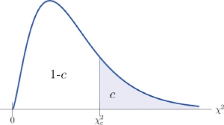
Then, the reasoning is the same as in any hypothesis test: if the test statistic is a large number, then the hypothesis of the theorem that request uniform distribution is wrong. The large chi-square statistic provide evidence against the null hypothesis. To determine the magnitude of numbers, we set a region of the chi-square distribution that we are not going to accept if the test statistic falls in this region. This region is called critical region or level of significance, and it is set at 1% (or 5% in other occasions). The number on the x-axis of the chi-square distribution to the right of which the critical region is found is called critical value, and it is easily determined by the tables of the distribution.

Figure 1

A chi-square distribution

The critical value of the chi-square distribution with 5 degrees of freedom, at 1% level of significance is 15.09, i.e., P(X>15.09)=0.01, while in R is written as:

qchisq(0.99,5)
[1] 15.08627

Indeed:

pchisq(15.09, 5)
[1] 0.9900154

or

pchisq(15.09, 5, lower.tail=FALSE)
[1] 0.009984625

The operations for the computation of $\chi^2$ test statistic can be easily executed in R .

With the command $chisq.test()$ the test is easily performed:

d1<-c(7,6,13,6,6,7)
> chisq.test(d1)

Chi-squared test for given probabilities

data: d1
X-squared = 5, df = 5, p-value = 0.4159

The probability of getting a chi-square test statistic greater than or equal to 5 is 0.4159. This region covers by far the threshold of 1%. (The critical value was 15.09 which is greater than the chi-square statistic 5). Consequently, the chi-square statistic falls in the acceptance region).

So, there is no evidence to reject the null hypothesis. Then, the outcomes of this experiment follow the uniform distribution, meaning that the die is fair.

Caution about the chi-square distribution: The chi-square distribution is a good approximation of the chi-square statistic, which is a necessary condition for the application of the test, as long as none of the expected numbers are smaller than 5. If there are categories with expected frequencies less than 5 then they must be combined in order to get all the expected frequencies greater than or equal to 5

In this experiment, we might be tempted to do a series of binomial tests for some of (or all) the individual numbers, from 1 to 6. For example, for the number 2, the probability of success (getting 2) is 1/6 and the probability of failure 5/6. The binomial formula will give the probability of getting 2, 6 times out of 45 tossing. Then, we must compare the obtained probability with the empirical probability of the experiment which is 6/45. But this solution is wrong

Test of independence and contingency tables

In the 1987 case of McCleskey vs.  Kemp, the Supreme Court upheld the constitutionality of Georgia’s death penalty, despite statistical evidence that blacks who murder whites are disproportionately sentenced to death. Here are some of the data considered by the court regarding 2475 Georgia murder convictions between 1973 and 1980

Table2

Data of murder convictions between 1973 and 1980

	BLACK DEFENDANT		WHITE DEFENDANT		TOTAL
	BLACK VICTIM	WHITE VICTIM	BLACK VICTIM	WHITE VICTIM
DEATH SENTENCE	18	50	2	58	128
NO DEATH SENTENCE	1420	178	62	687	2347
TOTAL	1438	228	64	745	2475

The data of the survey are classified in two ways: one way by the rows and one way by the columns. The table used to present the two-way labeled  data is called contingency table.

In this example, people are classified by sentence (death sentence and no death sentence) and by race identity of both the defendant and the victim. Thus, there are four categories when people are classified by columns:

BDBV : Black defendant and black victim
BDWV : Black defendant and white victim
WDBV : White defendant and black victim
WDWV : White defendant and white victim

It is interesting to find out if the two classifications are independent, i.e., if the race of defendant/victim influences the jury’s verdict.

This is representative example of the $\chi^2$ test of independence.

Usually, the null hypothesis sets the independence.

$H_0$: there is no relation between sentence and defendant/victim race

$H_1$: there is relation between sentence and defendant/victim race

Let us examine the hypothesis at the level of significance 1% of the chi-square distribution. Chi-square distribution always comes with degrees of freedom, which in the case of the two-way data is the product (rows-1)*(columns-1) for the rows and columns of the contingency table. In this experiment, the contingency table has 2 rows (Death sentence and no death sentence) and 4 columns. The associate chi-square distribution has 3 degrees of freedom.

The critical value that separates the 1% level of significance from the acceptance region in the chi-square distribution with (2-1)*(4-1)= 3 degrees of freedom is:

qchisq(0.99, 3)
[1] 11.34487

We can observe that overall, 5.17% (128/2475) of the defendants were sentenced to death. The percentages are somewhat smaller for white defendant/black victim , and somewhat larger for black defendant/white victim. Are these observed differences statistically significant, or might they be explained by sampling error?

If there are no large differences in reality and the unequal patterns are due to sampling error, so the null hypothesis is true, then we expect the percentage of defendant who are sentenced to death in each race category to be equal to 5.17%. Consequently, as there are 1438 BDBV cases, there must be (5.18%) *1438=74.37 BDBV cases sentenced to death. As there are 228 BDWV there must be (5.18%) *228=11.79 BDWV sentenced to death.

In that way, all the expected values can be computed following the rule: if the null hypothesis is true the expected value $e_{ij}$, meaning the expected value that is found in the i row and j column of the contingency table, is

$${expected\ value\ e}_{ij}=$$

$$=\ \frac{(total\ of\ the\ elements\ in\ the\ i\ row)\ast(total\ of\ the\ elemnts\ in\ the\ j\ column)}{2475}$$

Caution: Here we must carefully check that no expected number is smaller than 5.

Following the rational of the $\chi^2$ statistic:

$$\chi^2=\sum\frac{\left(observed-expected\right)^2}{expected}=$$

$$\frac{{(18-74.37)}^2}{74.37}+\frac{{(50-11.79)}^2}{11.79}+\ldots+\frac{{(687-706.47)}^2}{706.47} = 186.6$$

The chi-square statistic must be compared with the critical value.

Since 186.6 is bigger than 11.34487 , the results are highly significant and consequently the null hypothesis is rejected.

Therefore, there is relation between the sentence and the race defendant/victim.

The calculations can be made explicitly with R, by creating firstly a matrix $m$ whose columns and rows are the columns and rows of the contingency table.

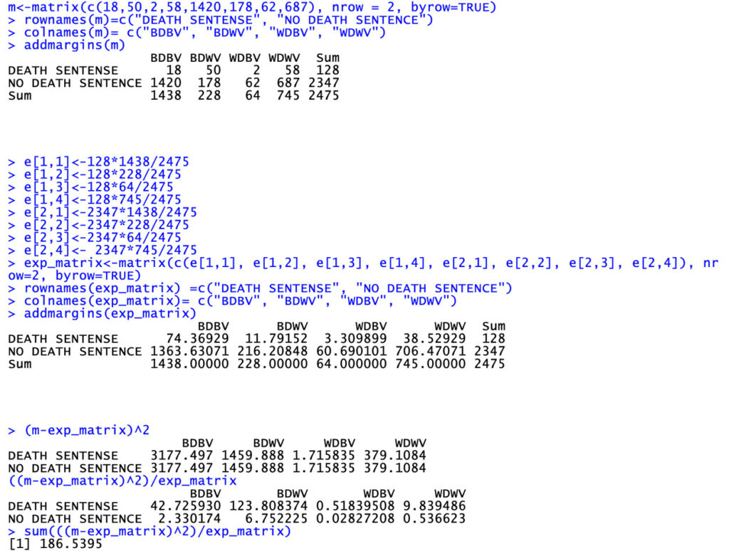
We may ask R to perform a chi-square test on the matrix m directly, and we get:

> chisq.test(m,3)

Pearson's Chi-squared test

data:  m
X-squared = 186.54, df = 3, p-value < 2.2e-16

In this case the statistical significance is proven by calculating the probability for the random variable to take on values greater than or equal to $\chi^2$ test statistic (given by the command $pchisq(186.54,\ 3,\ lower.tail=F)$ which is extremely smaller than the threshold of 0.01.

Fitting a Poisson Distribution

Fitting a distribution consists in finding a mathematical function which represents in a good way a statistical variable. If for example, we have some observations of a quantitative character and we wish to test if those observations come from a population with a specific distribution. In this case, a chi-square test is appropriate since we can assign to each observation an empirical probability based on the sample and an expected probability based on the theoretical distribution.

For example:

The manager of Goodyear Hotels studies the pattern of cancellations over a 90-day period. She observes the results shown in the following table:

Table 3

Hotel cancellation data

Number of cancellations	0	1	2	3	4	5	6	7	8	9
Number of days this number of cancellations was received	9	17	25	15	11	7	2	2	2	0

Are the data compatible with the hypothesis that the number of daily cancellations follows a Poisson distribution?

Firstly, the data must be imported in R. A vector of 90 data, each presenting a daily number of cancellation with their repetitions since the same number of cancellation can be observed several days is formed. Then, by using the command $table()$ we ask R to compute the frequencies:

Figure 2

Description and summary of the random variable “Number of Cancellations”

> d<-c(0,0,0,0,0,0,0,0,0,1,1,1,1,1,1,1,1,1,1,1,1,1,1,1,1,1, 2,2,2,2,2,2,2,2,2,2,2,2,2,2,2,2,2,2,2,2,2,2,2,2,2, 3,3,3,3,3,3,3,3,3,3,3,3,3,3,3, 4,4,4,4,4,4,4,4,4,4,4, 5,5,5,5,5,5,5,6,6,7,7,8,8)
> length(d)
[1] 90
> table(d)
d
9 1 2 3 4 5 6 7 8
9 17 25 15 11 7 2 2 2
> mean.x<-mean(d)
> mean.x
[1] 2.588889
> length(table(d))
[1] 9

Histograms and similar plots might be the best way to have an idea of the data pattern, before making any statistical test.

Figure 3

Histogram of the number of cancellations

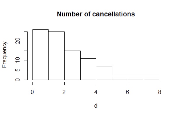
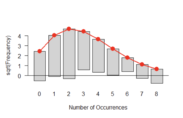
Obviously, the data have a shape remarkably similar to the shape of Poisson distribution.

We form the hypotheses:

$H_0$: the data came from a population that follows a Poisson distribution
$H_1$: the data did not come from a population that follows a Poisson distribution

We will test the null hypothesis at 1% level of significance of a chi-square distribution with 6 degrees of freedom. The choice of 6 will be explained later.

The critical value that separates the acceptance region of the distribution from the rejection region can be found using the command

$\ qchisq(0.01,\ degrees\ of\ freedom=6,\ lower.tail=F)$ and it is equal to 16.81

qchisq(0.01, 6, lower.tail=F)
[1] 16.81189

Using the $table(d)$ of the classified frequencies we can obtain the vector of frequencies with a simple algorithm:

> freq.obs<-vector()
> for(i in 1: length(table(d))) freq.obs[i]<-table(d)[[i]]
> freq.obs
[1] 9 17 25 15 11 7 2 2 2

Then, the vector of expected frequencies can be formed; its components indicate the frequency of the daily cancelation if the data were coming from a Poisson distribution whose parameter $\lambda$ is estimated by the mean of the sample, and so it is set at 2.6. It not unreasonable to estimate $\lambda$ by using the sample mean since $\lambda$ is the mean of the Poisson variable.

It is also known that the Poisson density function is given by:

$$f\left(x\right)=\frac{e^{-\lambda}\lambda^x}{x!} , for x=0,1,2,3,…$$

So, by using the above function we can find f(1)=\ P(X=1),\ f(2)=\ f(X=2),… Explicitly, f(1) is the probability of having 1 daily cancelation (the corresponding empirical probability is 17/90), f(2) is the probability of having two daily cancelations (the corresponding empirical probability equals 25/90). Multiplying each of these probabilities by 90 (we have 90 data) gives the expected frequency for each value of X.

Now, we can explain why the degrees of freedom of the chi-square distribution are 6: There are 9 categories but two of them have expected frequencies less than 5 , so we combine together. Then there are 8 categories, and consequently 8-1=7 degrees of freedom. One degree of freedom is lost because of the estimation of $\lambda$. Then by definition there must be 7-1 = 6 degrees of freedom

> freq.exp<-(dpois(0:max(d), lambda=mean(d)))*90
> freq.exp
[1] 6.759310 17.499102 22.651615 19.547505 12.651580 6.550707 2.826509 1.045360 0.338290

Then, the chi-square statistic is given by the formula:

$\chi^2=\sum_{i}^{8}\frac{{(observed-expected)}^2}{expected}$

R we easily perform the operations:

> chisq<- sum(((freq.obs-freq.exp)^2)/freq.exp)
> chisq
[1] 11.58077

The chi-square static is smaller than the critical value, which means that it is fallen in the acceptance region. Then, we do not have evidence to reject the null hypothesis. The variable “number of cancellations” follows a Poisson distribution.

Figure 4

Histogram of observed and expected data of the variable ‘Number of Cancellations”